Logistic Regression 💻

MATH 4780 / MSSC 5780 Regression Analysis

Dr. Cheng-Han Yu
Department of Mathematical and Statistical Sciences
Marquette University

Classification

Regression vs. Classification

• Linear regression assumes that the response \(Y\) is numerical.
• In many situations, \(Y\) is categorical.

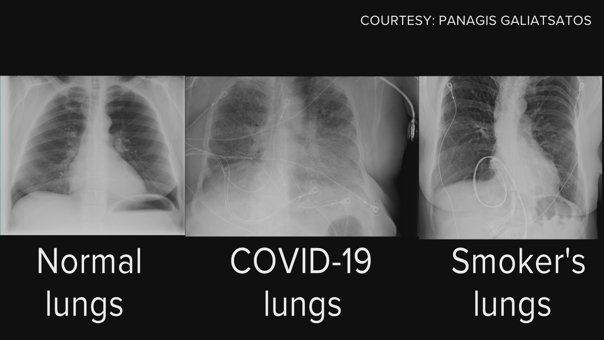
Normal vs. COVID vs. Smoking

fake news vs. true news

• A process of predicting categorical response is known as classification.

Regression Function \(f(x)\) vs. Classifier \(C(x)\)

Source: https://daviddalpiaz.github.io/r4sl/classification-overview.html

Classifiers

• Often, we first predict the probability of each of the categories of \(Y\), as a basis for making the classification (soft classifier).
• We discuss the classifiers
  • logistic
  • probit
  • complementary log-log
• Other classifiers include (MSSC 6250)
  • K-nearest neighbors
  • trees/random forests/boosting
  • support vector machines
  • convolutional neural networks, etc.

Classification Example

• Predict whether people will default on their credit card payment \((Y)\) yes or no, based on monthly credit card balance \((X)\).
• We use the (training) sample data \(\{(x_1, y_1), \dots, (x_n, y_n)\}\) to build a classifier.

Why Not Linear Regression?

\[Y =\begin{cases} 0 & \quad \text{if not default}\\ 1 & \quad \text{if default} \end{cases}\]

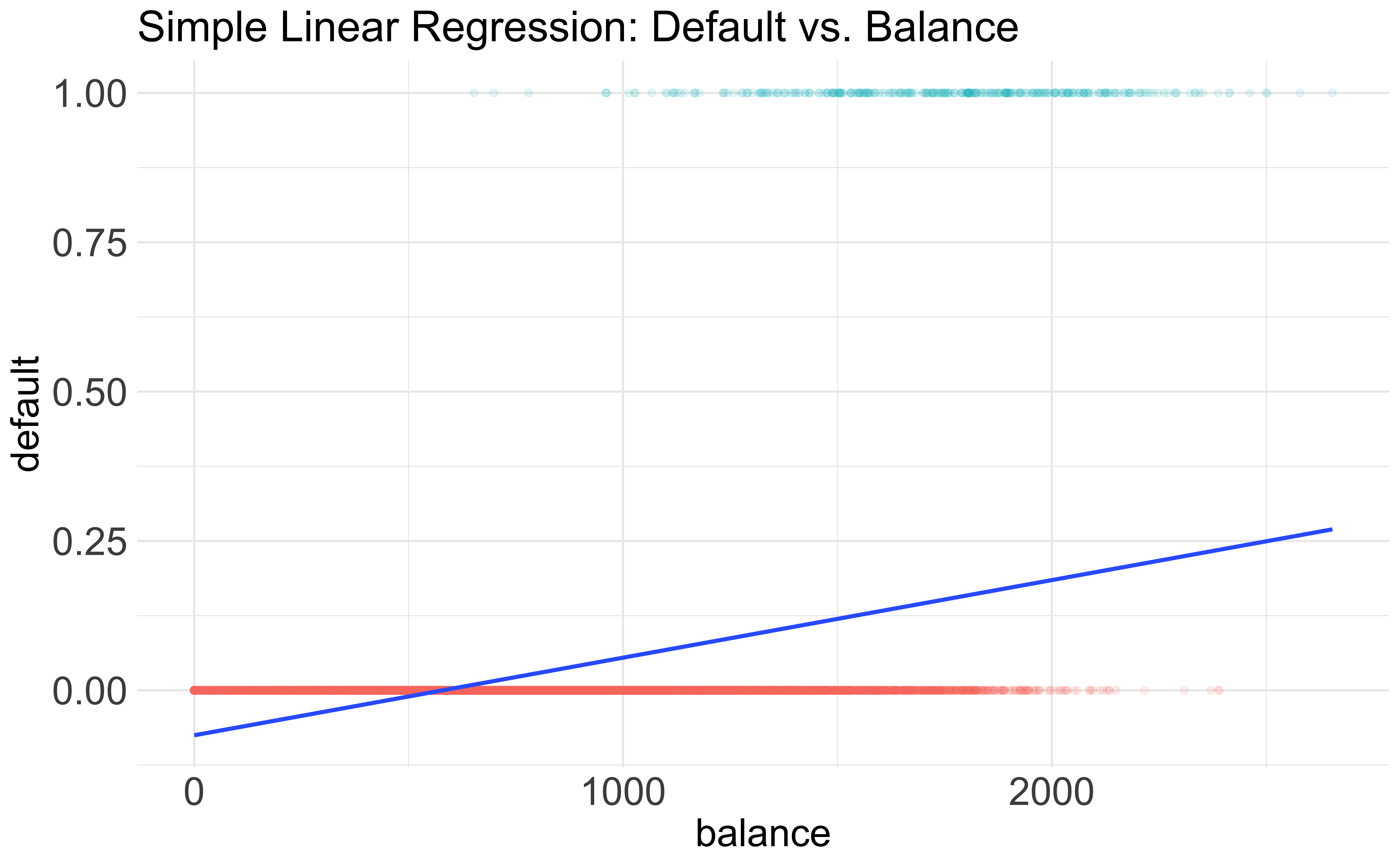
• \(Y = \beta_0 + \beta_1X + \epsilon\), \(\, X =\) credit card balance

What is the problem of this dummy variable approach?

• \(Y\) is categorical but coded as dummy variable or indicator variable
• Fit linear regression and treat it as a numerical variable.

Why Not Linear Regression?

• Some estimates are outside \([0, 1]\).

• The dummy variable approach \((Y = 0, 1)\) cannot be easily extended to \(Y\) with more than two categories.

Why Not Linear Regression?

• First predict the probability of each category of \(Y\).
• Predict probability of default using a S-shaped curve.

Often, we first predict the probability of each of the categories of \(Y\), as a basis for making the classification. - The predicted probability should be like a S-shaped curve that first is in [0, 1] interval. - Second, the predicted probability of being defualted is increasing in the credit card balance.

Logistic Regression

Binary Response

Binomial/Proportion Response

Multinomial Response (MSSC 6250)

• When we have several replicates of reposnse, meaning that we have several binary 0-1 outcomes of \(y\) at any given level of \(x\), we consider Binomial and Proportion Responses, that is the number of successes, or the proportion or the number of successes divided by the total number of trials or replicates.

Framing the Problem: Binary Responses

• Treat each outcome (default \((y = 1)\) and not default \((y = 0)\)) as success and failure arising from separate Bernoulli trials.

What is a Bernoulli trial?

• A Bernoulli trial is a special case of a binomial trial when the number of trials is \(m = 1\):
  • \(Bernoulli(\pi) = binomial(m = 1,\pi)\)
  • exactly two possible outcomes, “success” and “failure”
  • the probability of success \(\pi\) is constant

In the credit card example,

• do we have exactly two outcomes?
• do we have constant probability? \(P(y_1 = 1) = P(y_2 = 1) = \cdots = P(y_n = 1) = \pi?\)

• The idea is that we can treat \(Y\) as a categorical variable and each of its outcome is success or failure arising from separate Bernoulli trials
• And what is a Bernoulli trial? We talked about this when we talked about Binomial distribution, right?
• A Bernoulli trial is a random experiment with exactly two possible outcomes, “success” and “failure”, in which the probability of success is the same every time the experiment is conducted

Binary Responses with Nonconstant Probability

• Two outcomes: default \((y = 1)\) and not default \((y = 0)\)
• The probability of success \(\pi\) changes with the value of predictor \(X\)!
• With a different value of \(x_i\), each Bernoulli trial outcome \(y_i\) has a different probability of success \(\pi_i\):

\(y_i \mid x_i \stackrel{indep}{\sim} Bernoulli(\pi(x_i)) = binomial(m=1,\pi = \pi(x_i))\)

• Here, Each Bernoulli trial, with different value of \(x_i\), the trial outcome \(y_i\) can have a separate probability of success $ y_i x_i; p_i ∼ Bern(p_i) $.
• Actually this probability \(\pi_i\) is affected by the predictor \(x_i\). A different value of \(x\) will give you a different value of \(\pi\).
• Like linear regression, different value of \(x\) give us different mean of \(Y\)

• \(X =\) balance. \(x_1 = 2000\) has a larger \(\pi_1 = \pi(2000)\) than \(\pi_2 = \pi(500)\) with \(x_2 = 500\) because credit cards with a higher balance tend to be default.

Logistic Regression

• Logistic regression models a binary response \((Y)\) using predictors \(X_1, \dots, X_k\).
  • \(k = 1\): simple logistic regression
  • \(k > 1\): multiple logistic regression

• Logistic regression models a binary categorical outcome \((Y)\) using numerical and categorical predictors \(X_1, \dots, X_k\).

Instead of predicting \(y_i\) directly, we use the predictors to model its probability of success, \(\pi_i\).

But how?

• But remember, we are not predicting \(Y\) directly. Instead, our goal is to use predictors \(X_1, \dots, X_k\) to estimate the probability of success \(\pi\) of the Bernoulli variable \(Y\). And if \(\pi > threshold\), say 0.5, \(\hat{Y} = 1\), if \(\pi < threshold\), \(\hat{Y} = 0\).

• Transform \(\pi \in (0, 1)\) into another variable \(\eta \in (-\infty, \infty)\). Then construct a linear predictor on \(\eta\): \(\eta_i = \beta_0 + \beta_1x_i\)

• And the idea is that we transform \(p \in (0, 1)\) into another variable \(\eta \in (-\infty, \infty)\). So that we can reasonably fit a linear regression on \(\eta\).
  

• Logit function: For \(0 < \pi < 1\)

\[\eta = logit(\pi) = \ln\left(\frac{\pi}{1-\pi}\right)\]

• And the function that transforms \(p\) into \(\eta\) is the so called logit function defined as
• \(\eta = logit(p) = \ln\left(\frac{p}{1-p}\right)\)
• You see when \(p\) is approaching 0, p/1-p is also approaching 0, and so log of it is approaching -\(\infty\).
• When p is close to 1, p/1-p is close to \(\infty\), so is log because log is an increasing function.

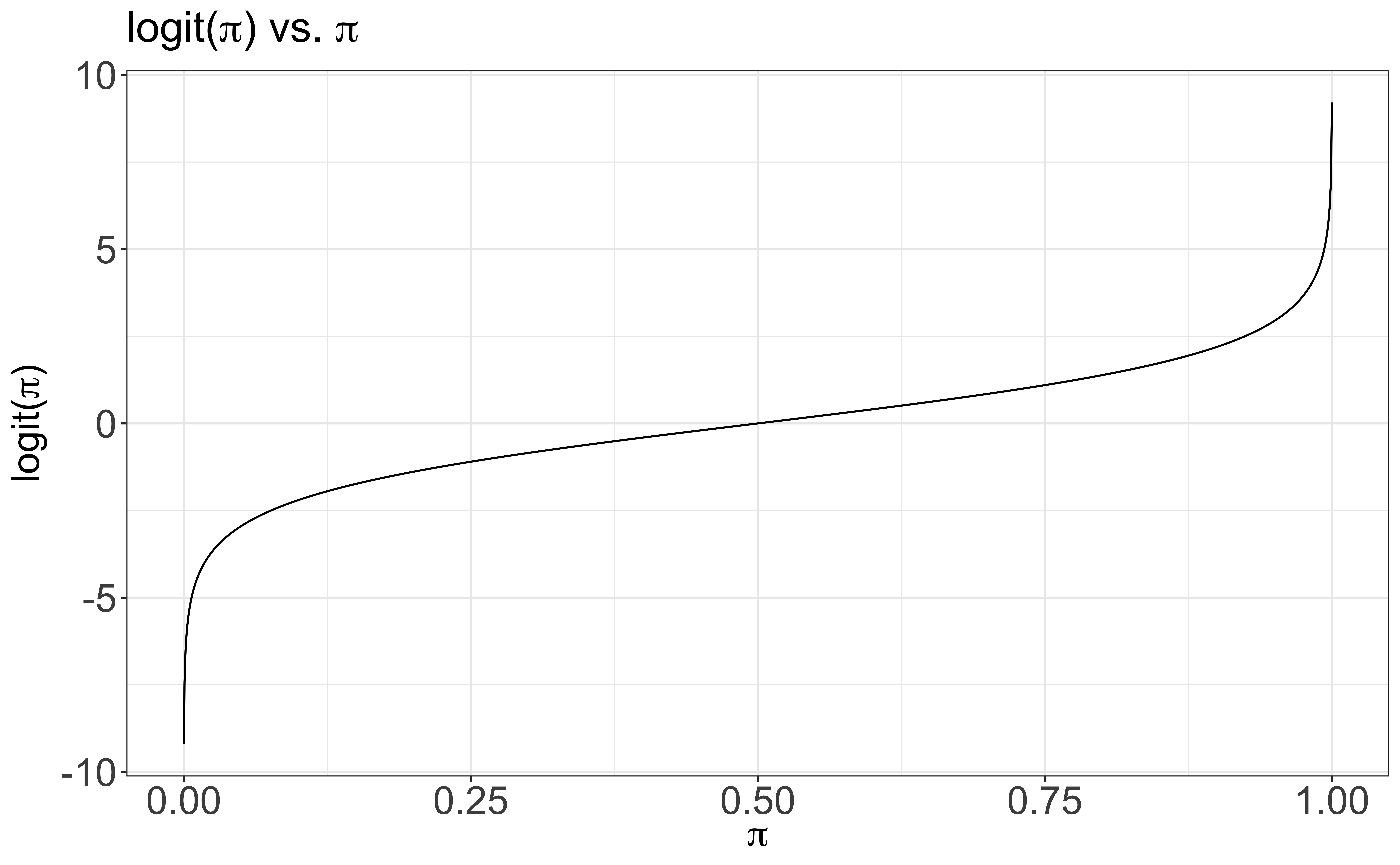
Logit function \(\eta = logit(\pi) = \ln\left(\frac{\pi}{1-\pi}\right)\)

• Here visualizes the logit function.
• It’s an one-to-one increasing function of \(\pi\) and so the inference on \(\eta\) can be transformed back to the inference of \(\pi\) with no problems.

Logistic Function

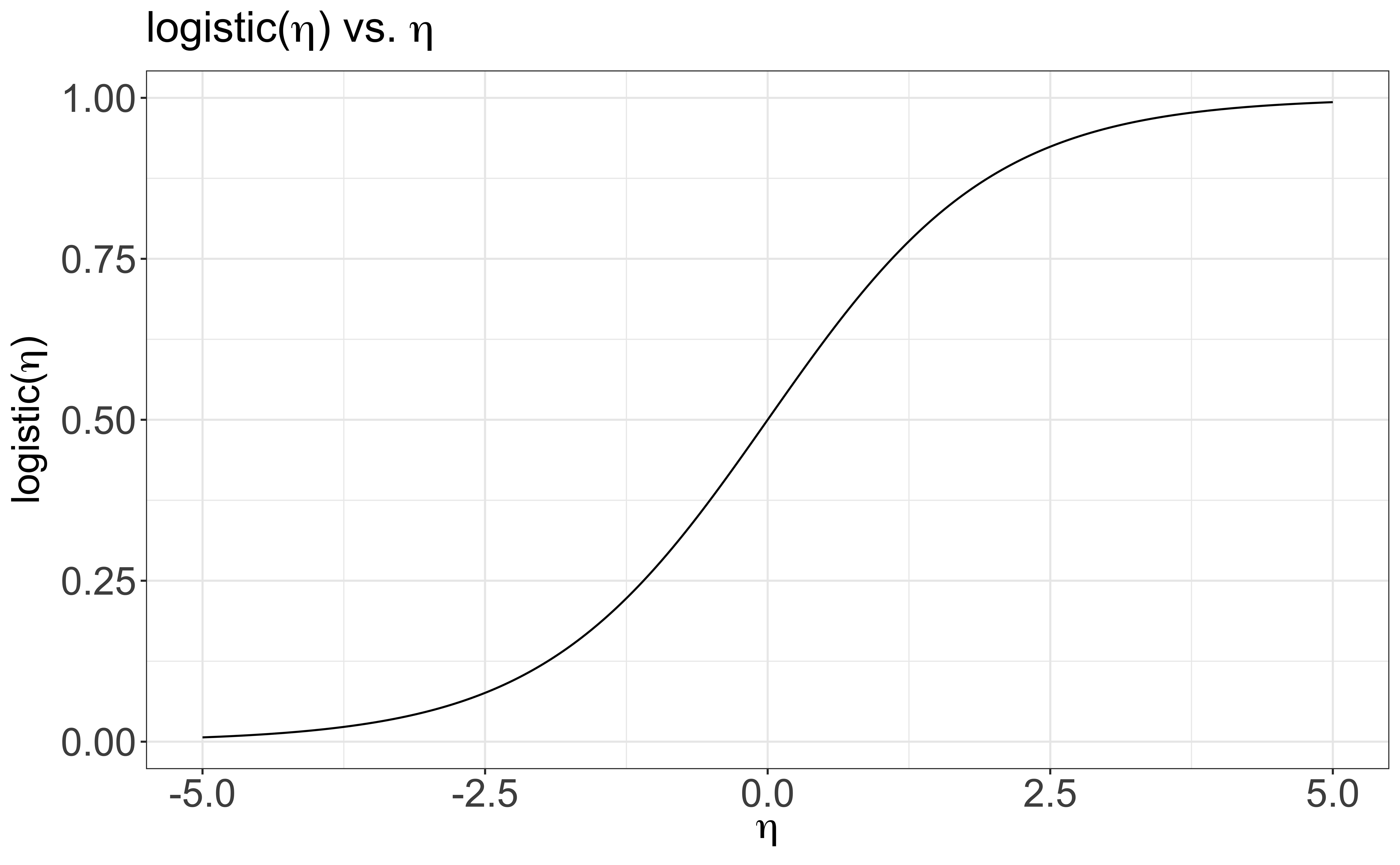
• The logit function \(\eta = logit(\pi) = \ln\left(\frac{\pi}{1-\pi}\right)\) takes a value \(\pi \in (0, 1)\) and maps it to a value \(\eta \in (-\infty, \infty)\).
• Logistic function: \[\pi = logistic(\eta) = \frac{\exp(\eta)}{1+\exp(\eta)} = \frac{1}{1+\exp(-\eta)} \in (0, 1)\]
• The logistic function takes a value \(\eta \in (-\infty, \infty)\) and maps it to a value \(\pi \in (0, 1)\).

• So once \(\eta\) is estimated by the linear regression, we use the logistic function to transform \(\eta\) back to the probability.

• The logit function \(\eta = logit(\pi) = \ln\left(\frac{\pi}{1-\pi}\right)\) takes a value \(\pi \in (0, 1)\) and maps it to a value \(\eta \in (-\infty, \infty)\).
• Inverse logit (logistic) function: \[\pi = logistic(\eta) = \frac{\exp(\eta)}{1+\exp(\eta)} = \frac{1}{1+\exp(-\eta)} \in (0, 1)\]
• The inverse logit function takes a value \(\eta\) between \(-\infty\) and \(\infty\) and maps it to a value \(\pi\) between 0 and 1.

Logistic Function \(\pi = logistic(\eta) = \frac{\exp(\eta)}{1+\exp(\eta)}\)

• We are almost there. The value of logistic function is what we need for predicting the probability that \(Y = 1\).
• Given any value of \(\eta\), there is a corresponding estimated probability.
• So if we can use our predictors to get eta first, then we can use the eta to predict the probability of \(Y\) being equal to when the predictors are at the level for getting \(\eta\).

Simple Logistic Regression Model

For \(i = 1, \dots, n\) and with one predictor \(X\): \[(Y_i \mid X = x_i) \stackrel{indep}{\sim} Bernoulli(\pi(x_i))\] \[\text{logit}(\pi_i) = \ln \left( \frac{\pi(x_i)}{1 - \pi(x_i)} \right) = \eta_i = \beta_0+\beta_1 x_{i}\]

• with sample size \(n\) and with \(k\) predictors, we have the logistic regression model like this
• First, we have a probability distribution Bernoulli describing how the outcome or response data are generated.
  • \(Y_i \mid {\bf x}_i; \pi_i \sim \text{Bern}(p_i)\), \({\bf x}_i = (x_{1,i}, \cdots, x_{k,i})\), \(i = 1, \dots, n\)
• Then we have a link function, logit function, that relates the linear regression to the parameter of the outcome distribution, which is the parameter \(p\), the probability of success in the Bernoulli distribution.
  • \(\text{logit}(\pi_i) = \eta_i = \beta_0+\beta_1 x_{1,i} + \cdots + \beta_k x_{k,i}\)

Once we get the estimates \(\hat{\beta}_0\) and \(\hat{\beta}_1\), \[\small \hat{\pi}_i = \frac{\exp(\hat{\beta}_0+\hat{\beta}_1 x_{i} )}{1+\exp(\hat{\beta}_0+\hat{\beta}_1 x_{i})} = \frac{1}{1+\exp(-\hat{\beta}_0-\hat{\beta}_1 x_{i}))}\]

.alert[ In general, if \(E(Y_i) = \mu_i\), \(g(\mu_i) = \eta_i = {\bf x}_i'\boldsymbol \beta\), \(\mu_i= g^{-1}(\eta_i) = g^{-1}({\bf x}_i'\boldsymbol \beta)\). Here \(\mu_i = \pi_i\), \(g(\cdot) = \text{logit}(\cdot)\).] - From which we get the probability of success derived by the logistic function \[E(y_i) = \pi_i = \frac{\exp(\beta_0+\beta_1 x_{1,i} + \cdots + \beta_k x_{k,i})}{1+\exp(\beta_0+\beta_1 x_{1,i} + \cdots + \beta_k x_{k,i})}\] or the predicted probability is the one that replaces \(\beta\) with estimates \(b\). \[\hat{\pi}_i = \frac{\exp(\hat{\beta}_0+\hat{\beta}_1 x_{1,i} + \cdots + \hat{\beta}_k x_{k,i})}{1+\exp(\hat{\beta}_0+\hat{\beta}_1 x_{1,i} + \cdots + \hat{\beta}_k x_{k,i})}\]

R Lab Credit Card Default

library(ISLR2)
head(Default, 10)

   default student balance income
1       No      No     730  44362
2       No     Yes     817  12106
3       No      No    1074  31767
4       No      No     529  35704
5       No      No     786  38463
6       No     Yes     920   7492
7       No      No     826  24905
8       No     Yes     809  17600
9       No      No    1161  37469
10      No      No       0  29275

str(Default)

'data.frame':   10000 obs. of  4 variables:
 $ default: Factor w/ 2 levels "No","Yes": 1 1 1 1 1 1 1 1 1 1 ...
 $ student: Factor w/ 2 levels "No","Yes": 1 2 1 1 1 2 1 2 1 1 ...
 $ balance: num  730 817 1074 529 786 ...
 $ income : num  44362 12106 31767 35704 38463 ...

table(Default$default)

  No  Yes 
9667  333 

table(Default$student)

  No  Yes 
7056 2944 

summary(Default$balance)

   Min. 1st Qu.  Median    Mean 3rd Qu.    Max. 
      0     482     824     835    1166    2654 

summary(Default$income)

   Min. 1st Qu.  Median    Mean 3rd Qu.    Max. 
    772   21340   34553   33517   43808   73554 

R Lab Simple Logistic Regression

library(tidyverse)
Default |>  
    group_by(default) |>
    summarise(avg_balance = mean(balance))

# A tibble: 2 × 2
  default avg_balance
  <fct>         <dbl>
1 No             804.
2 Yes           1748.

logit_fit <- glm(default ~ balance, data = Default, family = binomial)
summ_logit_fit <- summary(logit_fit)
summ_logit_fit$coefficients

            Estimate Std. Error z value  Pr(>|z|)
(Intercept) -10.6513    0.36116   -29.5 3.62e-191
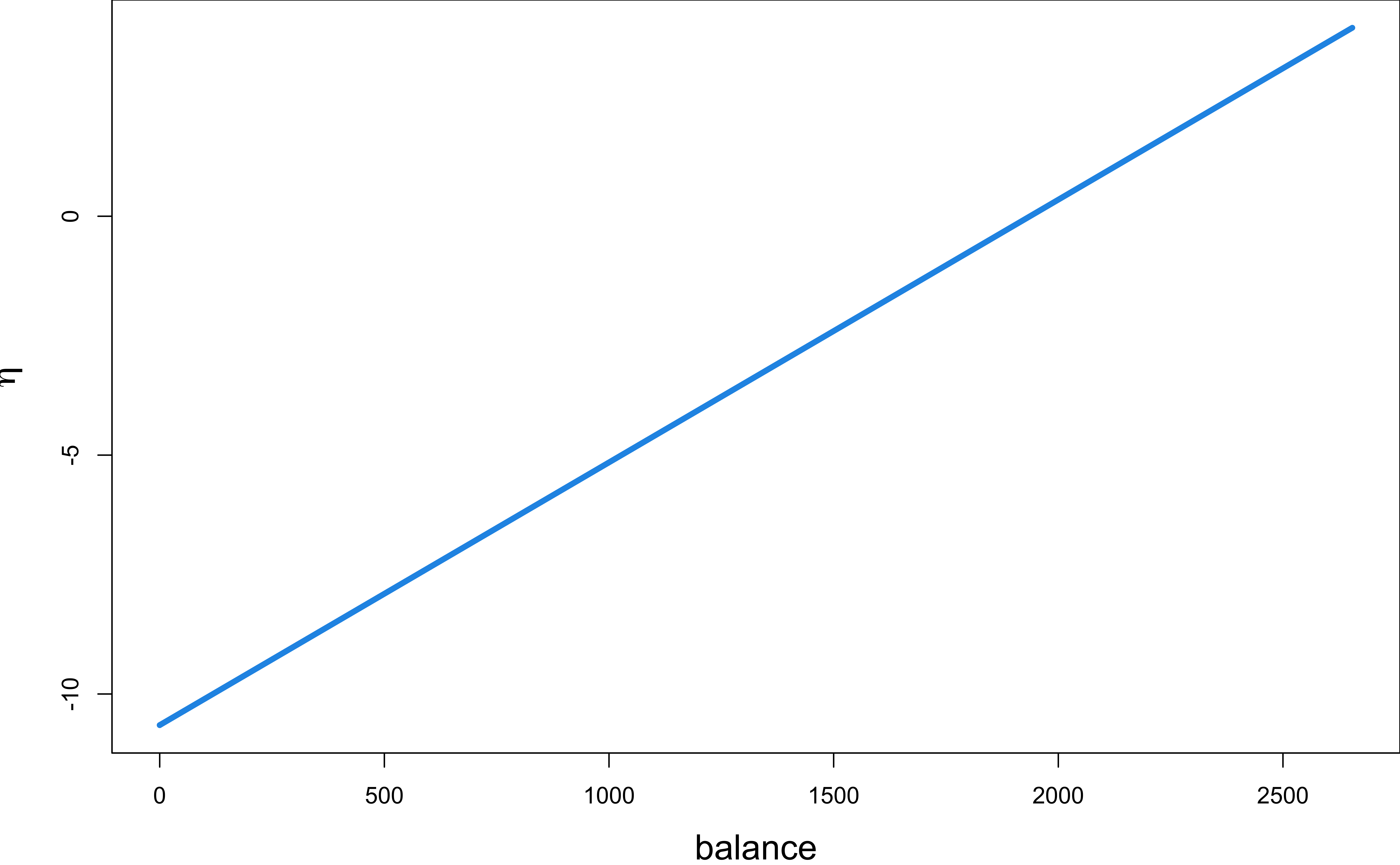
balance       0.0055    0.00022    25.0 1.98e-137

• \(\hat{\eta} = \text{logit}(\hat{\pi}) = \ln \left( \frac{\hat{\pi}}{1 - \hat{\pi}}\right) = -10.651 + 0.0055 \times \text{balance}\)

\(\eta\) vs. \(x\)

• \(\hat{\eta} = \text{logit}(\hat{\pi}) = \ln \left( \frac{\hat{\pi}}{1 - \hat{\pi}}\right) = -10.651 + 0.0055 \times \text{balance}\)

Interpretation of Coefficients

The ratio \(\frac{\pi}{1-\pi} \in (0, \infty)\) is called the odds of some event.

• Example: If 1 in 5 people will default, the odds is 1/4 since \(\pi = 0.2\) implies an odds of \(0.2/(1−0.2) = 1/4\).

\[\ln \left( \frac{\pi(x)}{1 - \pi(x)} \right)= \beta_0 + \beta_1x\] - Increasing \(x\) by one unit changes the log-odds by \(\beta_1\), or it multiplies the odds by \(e^{\beta_1}\).

• \(\beta_1\) does not correspond to the change in \(\pi(x)\) associated with a one-unit increase in \(x\).
• \(\beta_1\) is the change in log odds associated with one-unit increase in \(x\).

R Lab Interpretation of Coefficients

            Estimate Std. Error z value  Pr(>|z|)
(Intercept) -10.6513    0.36116   -29.5 3.62e-191
balance       0.0055    0.00022    25.0 1.98e-137

• \(\hat{\eta} = \text{logit}(\hat{\pi}) = \ln \left( \frac{\hat{\pi}}{1 - \hat{\pi}}\right) = -10.651 + 0.0055 \times \text{balance}\)

• \(\hat{\eta}(x) = \hat{\beta}_0 + \hat{\beta}_1x\)
• \(\hat{\eta}(x+1) = \hat{\beta}_0 + \hat{\beta}_1(x+1)\)
• \(\hat{\eta}(x+1) - \hat{\eta}(x) = \hat{\beta}_1 = \ln(\text{odds}_{x+1}) - \ln(\text{odds}_{x})\)
• One-unit increase in balance increases the log odds of default by 0.0055 units.

• The odds ratio, \(\widehat{OR} = \frac{\text{odds}_{x+1}}{\text{odds}_{x}} = e^{\hat{\beta}_1} = e^{0.0055} = 1.005515\).

• The odds of default increases by 0.55% with additional one unit of credit card balance.

Probability Curve

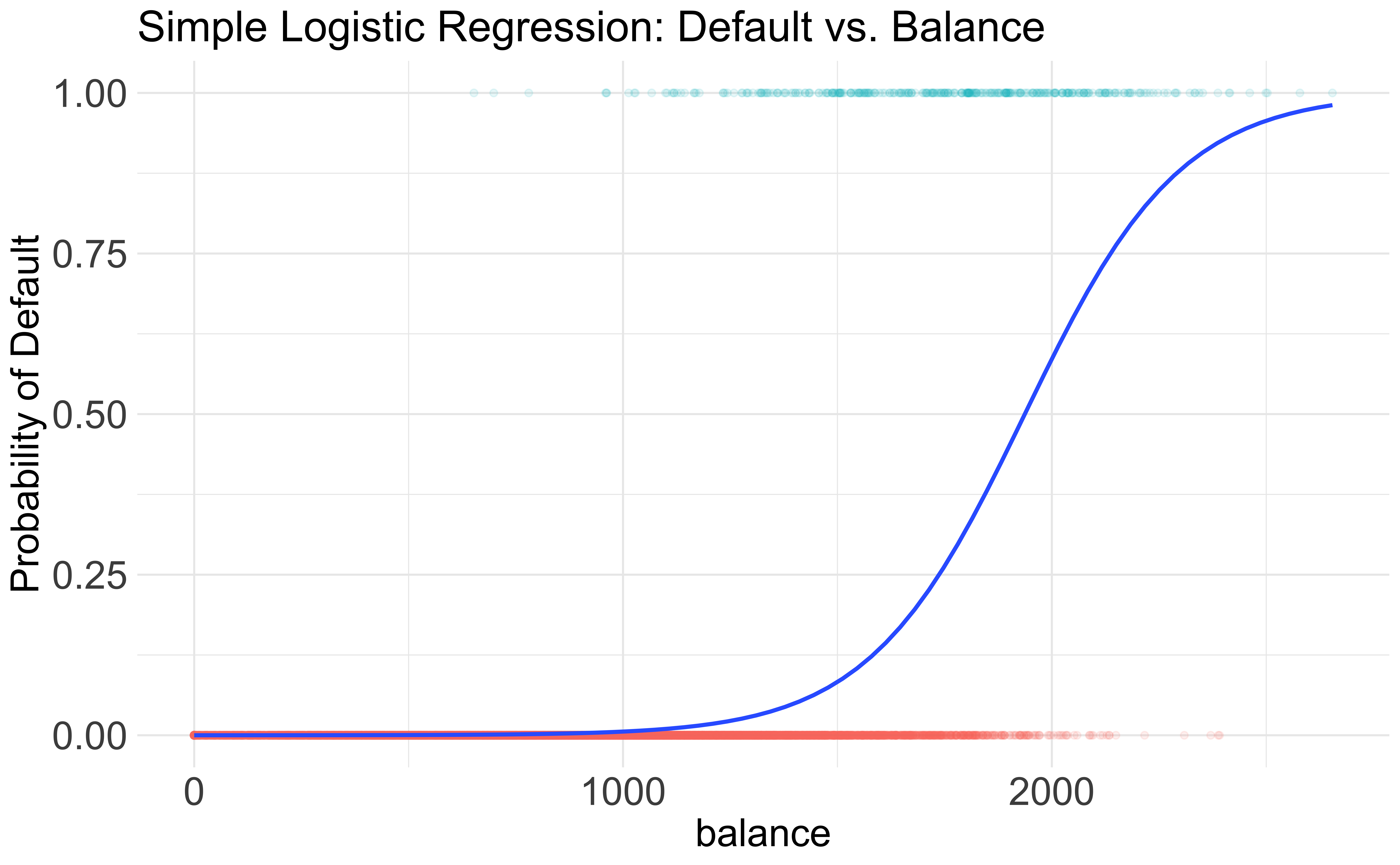
• The relationship between \(\pi(x)\) and \(x\) is not linear! \[\pi(x) = \frac{\exp(\beta_0+\beta_1 x)}{1+\exp(\beta_0+\beta_1 x)}\]
• The amount that \(\pi(x)\) changes due to a one-unit change in \(x\) depends on the current value of \(x\).
• Regardless of the value of \(x\), if \(\beta_1 > 0\), increasing \(x\) will be increasing \(\pi(x)\).

Pr(default) When Balance is 2000

\[\log\left(\frac{\hat{\pi}}{1-\hat{\pi}}\right) = -10.651+0.0055\times 2000\]

\[ \hat{\pi} = \frac{1}{1+\exp(-(-10.651+0.0055 \times 2000)} = 0.586\]

pi_hat <- predict(logit_fit, type = "response")
eta_hat <- predict(logit_fit, type = "link")  ## default gives us b0 + b1*x
predict(logit_fit, newdata = data.frame(balance = 2000), type = "response")

    1 
0.586 

Probability Curve

What is the probability of default when the balance is 500? What about balance 2500?

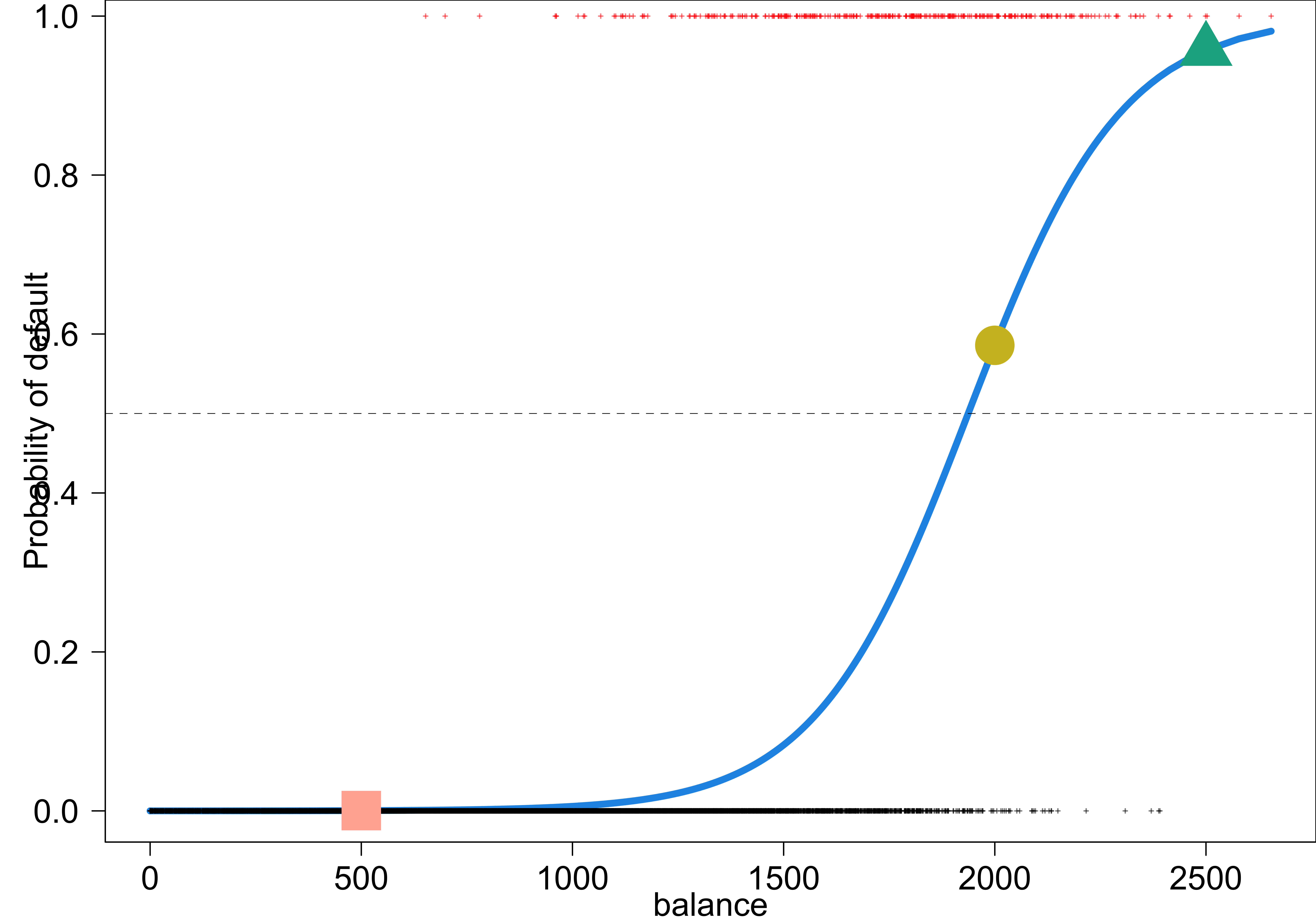
• 500 balance: Pr(default) = 0
• 2000 balance, Pr(default) = 0.59
• 2500 balance, Pr(default) = 0.96

Multiple Logistic Regression Model

For \(i = 1, \dots, n\) and with \(k\) predictors: \[Y_i \mid \pi_i({\bf x}_i) \stackrel{indep}{\sim} \text{Bernoulli}(\pi_i), \quad {\bf x}_i' = (x_{i1}, \dots, x_{ik})\] \[\text{logit}(\pi_i) = \ln \left( \frac{\pi_i}{1 - \pi_i} \right) = \eta_i = \beta_0+\beta_1 x_{i1} + \cdots + \beta_k x_{ik} = {\bf x}_i'\boldsymbol \beta\]

• The \(\text{logit}(\pi_i)\) is a link function that links the linear predictor and the mean of \(Y_i\).

• with sample size \(n\) and with \(k\) predictors, we have the logistic regression model like this
• First, we have a probability distribution Bernoulli describing how the outcome or response data are generated.
  • \(Y_i \mid {\bf x}_i; \pi_i \sim \text{Bern}(p_i)\), \({\bf x}_i = (x_{1,i}, \cdots, x_{k,i})\), \(i = 1, \dots, n\)
• Then we have a link function, logit function, that relates the linear regression to the parameter of the outcome distribution, which is the parameter \(p\), the probability of success in the Bernoulli distribution.
• \(\text{logit}(\pi_i) = \eta_i = \beta_0+\beta_1 x_{1,i} + \cdots + \beta_k x_{k,i}\)

\[\small E(Y_i) = \pi_i = \frac{\exp(\eta_i)}{1 + \exp(\eta_i)} = \frac{\exp(\beta_0+\beta_1 x_{i1} + \cdots + \beta_k x_{ik})}{1+\exp(\beta_0+\beta_1 x_{i1} + \cdots + \beta_k x_{ik})} = \frac{\exp( {\bf x}_i'\boldsymbol \beta)}{1 + \exp({\bf x}_i'\boldsymbol \beta)}\] \[\small \hat{\pi}_i = \frac{\exp(\hat{\beta}_0+\hat{\beta}_1 x_{i1} + \cdots + \hat{\beta}_k x_{ik})}{1+\exp(\hat{\beta}_0+\hat{\beta}_1 x_{i1} + \cdots + \hat{\beta}_k x_{ik})}\]

• From which we get the probability of success derived by the logistic function \[E(y_i) = \pi_i = \frac{\exp(\beta_0+\beta_1 x_{1,i} + \cdots + \beta_k x_{k,i})}{1+\exp(\beta_0+\beta_1 x_{1,i} + \cdots + \beta_k x_{k,i})}\] or the predicted probability is the one that replaces \(\beta\) with estimates \(b\). \[\hat{\pi}_i = \frac{\exp(\hat{\beta}_0+\hat{\beta}_1 x_{1,i} + \cdots + \hat{\beta}_k x_{k,i})}{1+\exp(\hat{\beta}_0+\hat{\beta}_1 x_{1,i} + \cdots + \hat{\beta}_k x_{k,i})}\]

In general, if \(E(Y_i) = \mu_i\), \(g(\mu_i) = \eta_i = {\bf x}_i'\boldsymbol \beta\), \(\mu_i= g^{-1}(\eta_i) = g^{-1}({\bf x}_i'\boldsymbol \beta)\). Here \(\mu_i = \pi_i\), \(g(\cdot) = \text{logit}(\cdot)\).

R Lab Multiple Logistic Regression

multi_logit_fit <- glm(default ~ balance + I(income/1000), data = Default, 
                       family = binomial)
summ_multi_logit_fit <- summary(multi_logit_fit)
summ_multi_logit_fit$coefficients

                Estimate Std. Error z value  Pr(>|z|)
(Intercept)    -11.54047   0.434756  -26.54 2.96e-155
balance          0.00565   0.000227   24.84 3.64e-136
I(income/1000)   0.02081   0.004985    4.17  2.99e-05

• \(\hat{\eta} = \text{logit}(\hat{\pi}) = \ln \left( \frac{\hat{\pi}}{1 - \hat{\pi}}\right) = -11.54 + 0.0056 \times \text{balance} + 0.021 \times \text{income}\)

• One with a credit card balance of $1,500 and an income of $40,000 has an estimated probability of default of \[\hat{\pi} = \frac{1}{1+ \exp(-(-11.54 + 0.0056(1500) + 0.021(40)))} = 0.091\]

Why we multiply the income coefficient by 40, rather than 40,000?

Multiple Binary Outcomes

• So far we consider only one binary outcome for each combination of predictors.

• Often we have repeated observations or trials at each level of the regressors.

• Originally, at \(X = x_i\), we have one single observation \(y_i = 0\) or \(1\).

• Now, at \(X = x_i\), we have \(m_i\) trials and \(y_i\) of them are ones (successes).

• Let \(y_{i,j}\) be an indicator (Bernoulli) variable taking value \(0\) or \(1\) for the \(j\)-th trial at \(x_i\).

• \(y_i = y_{i,1} + y_{i,2} + \cdots + y_{i, m_i} = \sum_{j=1}^{m_i} y_{i,j}\).

Bernoulli to binomial

• Example:
  • 4 dosages of a combination of drugs, \((10, 15, 20, 25)\)
  • 10 patients for each dosage
  • see how dosage level affects the number of cure of some disease among patients
• \(i = 1, 2, 3, 4\), \(x_1 = 10, \dots, x_4 = 25\), \(n = 4\)
• \(m_i = 10\) for each \(i\)
• \(y_i = y_{i, 1} + \cdots + y_{i, 10}\) is the number of patients whose disease is cured at \(i\)-th dosage, where \(y_{i, j} = 1\) if \(j\)-th patient is cured, \(0\) otherwise.

What is our response and any distribution can be used to model that?

• So far we consider only one binary outcome for each combination of predictors, and the response is Bernoulli distributed.
• Often we have more than one or repeated observations or trials at each level of the \(x\) variables.
• Originally, at \(X = x_i\), we have one single observation \(y_i = 0\) or \(1\). Now, at \(X = x_i\), we have \(m_i\) trials and \(s_i\) of them are ones (successes).
  • Regressors are dosages of a combination of drugs and a success represents a cure of a disease.

Binomial Responses

• The responses \(Y_i \sim binomial(m_i, \pi_i)\).

• Assume \(Y_1, Y_2, \dots, Y_n\) are independent. ( \(m_i\) trials, \(y_{i, 1}, \dots, y_{i, m_i}\), are independent too by the definition of a binomial experiment )

Number of trials	Number of successes	Regressors
\(m_1\)	\(y_1\)	\(x_{11}, x_{12}, \dots, x_{1k}\)
\(m_2\)	\(y_2\)	\(x_{21}, x_{22}, \dots, x_{2k}\)
\(\vdots\)	\(\vdots\)	\(\vdots\)
\(m_n\)	\(y_n\)	\(x_{n1}, x_{n2}, \dots, x_{nk}\)

• \(Pr(Y_i = y_i) = {m_i \choose y_i} \pi_i^{y_i} (1-\pi_i)^{m_i - y_i}\)
• \(E[Y_i] = m_i\pi_i\)
• \(\mathrm{Var}[Y_i] = m_i\pi_i(1-\pi_i)\)

R Lab Strength of Fastener (LRA 13.3)

• The compressive strength of an alloy fastener used in aircraft construction is being studied.

• Ten loads were selected over the range 2500 – 4300 psi and a number of fasteners were tested at those loads.

• The numbers of fasteners failing at each load were recorded.

fastener <- read.csv("./data/data-prob-13-3.csv")
colnames(fastener) <- c("load", "m", "y")
fastener

   load   m  y
1  2500  50 10
2  2700  70 17
3  2900 100 30
4  3100  60 21
5  3300  40 18
6  3500  85 43
7  3700  90 54
8  3900  50 33
9  4100  80 60
10 4300  65 51

R Lab Binomial Response Logistic Regression

binom_fit <- glm(cbind(y, m - y) ~ load,  #<<
                 data = fastener, family = binomial)
binom_summ <- summary(binom_fit)
binom_summ$coef

            Estimate Std. Error z value Pr(>|z|)
(Intercept) -5.33971   0.545693   -9.79 1.30e-22
load         0.00155   0.000158    9.83 8.45e-23

\[\hat{\pi} = \frac{e^{-5.34 + 0.0015x}}{1 + e^{-5.34 + 0.0015x}}\]

The complete test data are shown below.

Evaluation Metrics

• OK we learn the logistic regression model, we know how to do estimation using R, and now it’s time to introduce some evaluation metrics or performance measures for classification problems.
• Given a predicted probability, we may correctly classify the label, or mis-classify the label.
• And here we are going to talk about two metrics sensitivity and specificity.
• It’s hard for me to remember which is which, so I always open their Wiki page when I am working on them.
• All right let’s see what they are.

Sensitivity and Specificity

	0	1
Labeled 0	True Negative (TN)	False Negative (FN)
Labeled 1	False Positive (FP)	True Positive (TP)

• Sensitivity (True Positive Rate) \(= P( \text{Labeled 1} \mid \text{1}) = \frac{TP}{TP+FN}\)

• Specificity (True Negative Rate) \(= P( \text{Labeled 0} \mid \text{0}) = \frac{TN}{FP+TN}\)

• Accuracy \(= \frac{TP + TN}{TP+FN+FP+TN}\)

• More on Wiki page

R Lab Confusion Matrix

pred_prob <- predict(logit_fit, type = "response")
table(pred_prob > 0.5, Default$default)

       
          No  Yes
  FALSE 9625  233
  TRUE    42  100

• Packages:
  • caret package (Classification And REgression Training)
  • yardstick of tidymodels

caret::confusionMatrix()
yardstick::conf_mat()

• caret package (Classification And REgression Training) provides tools for predictive modeling.

## Classification And REgression Training
library(caret) 
caret::confusionMatrix(data = a factor of predicted classes, 
                       reference = a factor of classes to be used as the true results)

• yardstick is a package of tidymodels for estimating how well models are working.

yardstick::conf_mat(data = a data frame, 
                    truth = true class column that is a factor,
                    estimate = predicted class column that is a factor)

R Lab Receiver Operating Characteristic (ROC) Curve

• Receiver operating characteristic (ROC) curve plots True Positive Rate (Sensitivity) vs. False Positive Rate (1 - Specificity)
• Packages: ROCR, pROC, yardstick::roc_curve()

library(ROCR)

# create an object of class prediction 
pred <- ROCR::prediction(
    predictions = pred_prob, 
    labels = Default$default)

# calculates the ROC curve
roc <- ROCR::performance(
    prediction.obj = pred, 
    measure = "tpr",
    x.measure = "fpr")

plot(roc, colorize = TRUE)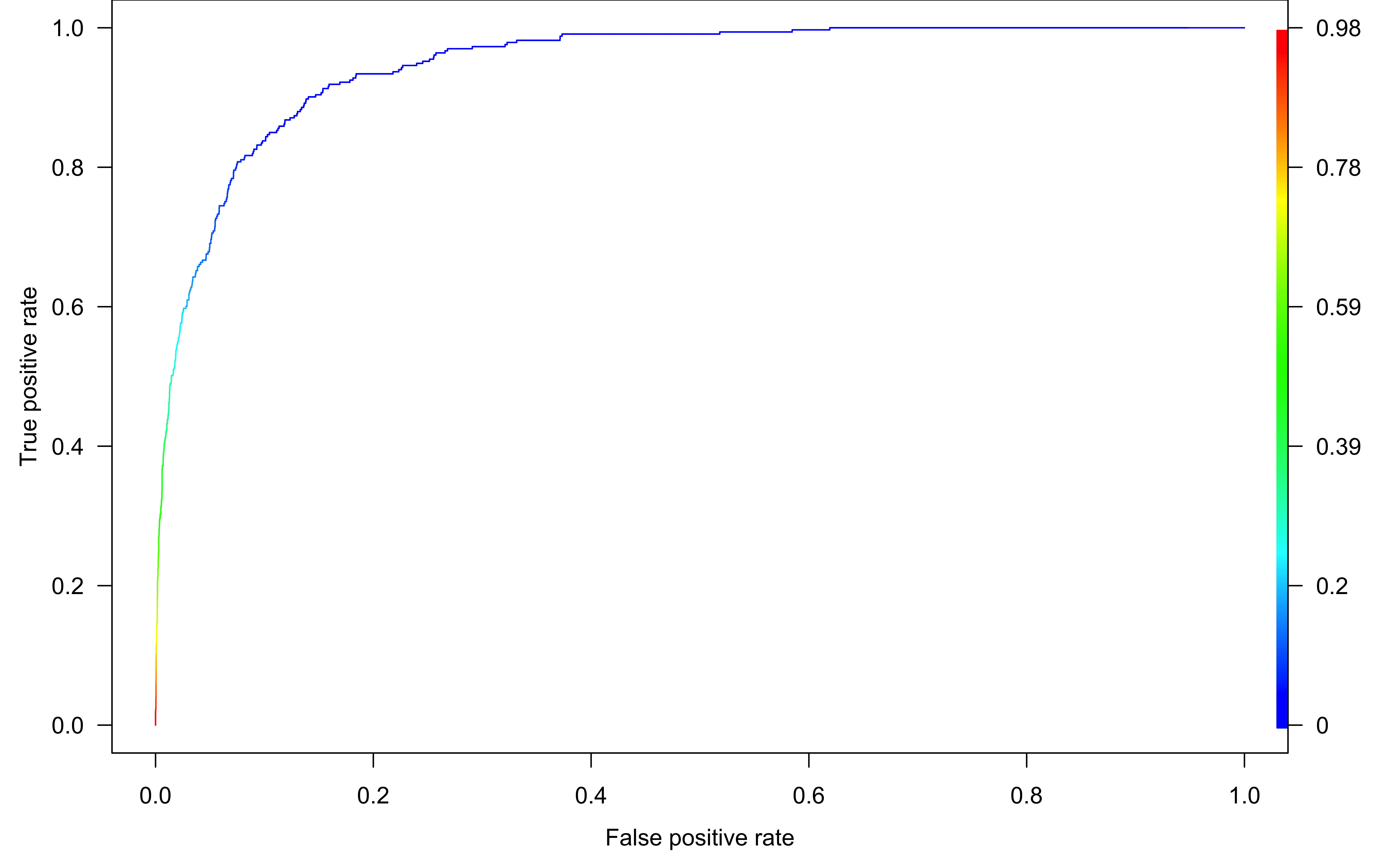

https://rviews.rstudio.com/2019/03/01/some-r-packages-for-roc-curves/ .footnote[ .small[ ⁺Originally developed for operators of military radar receivers, hence the name.]]

R Lab Area Under Curve (AUC)

Find the area under the curve:

## object of class 'performance'

auc <- ROCR::performance(
    prediction.obj = pred, 
    measure = "auc")
auc@y.values

[[1]]
[1] 0.948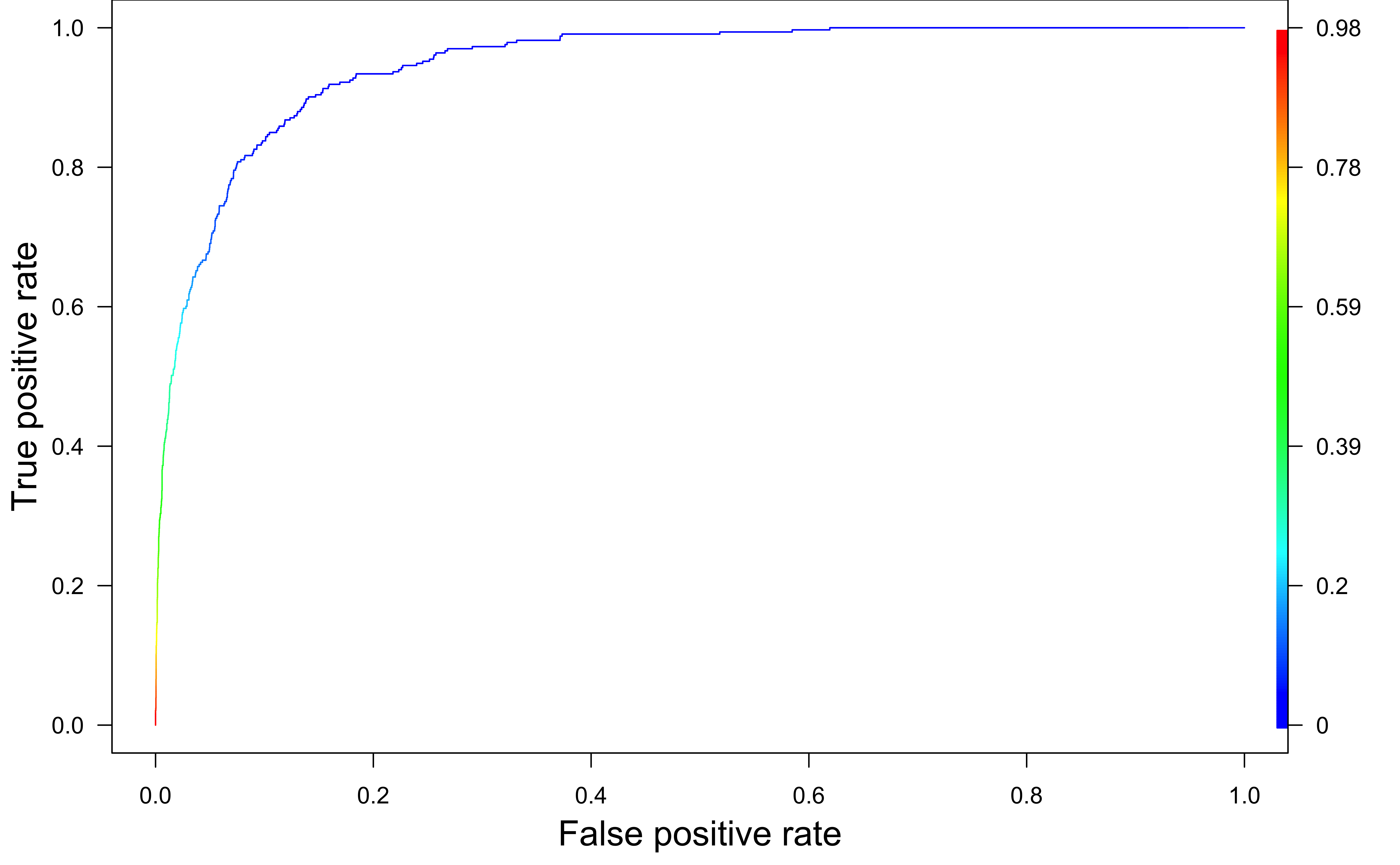

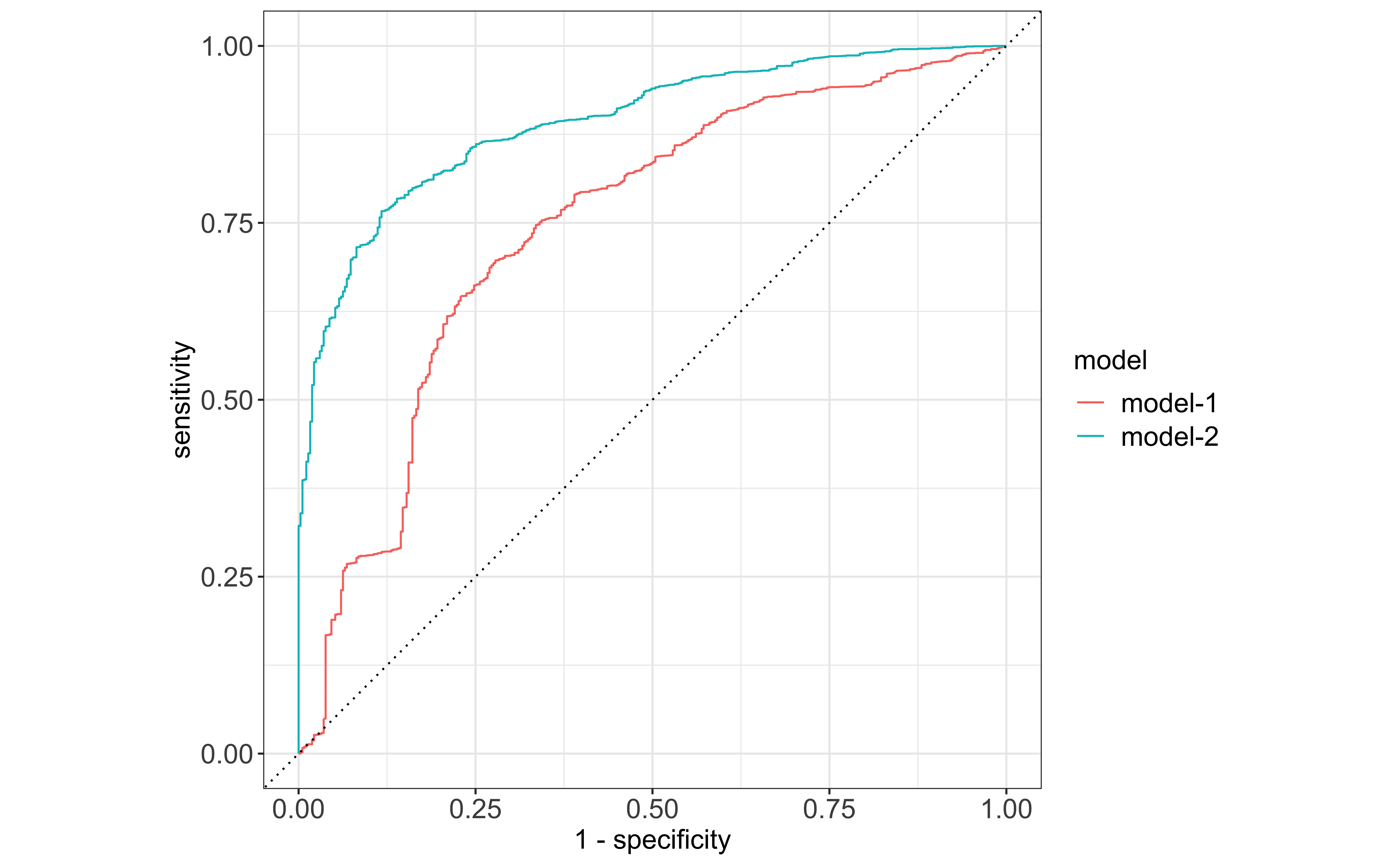
R Lab ROC Curve Comparison

Which model performs better?

Remember! Compare the candidates using the test data.