Model Building, Selection and Validation

MATH 4780 / MSSC 5780 Regression Analysis

Dr. Cheng-Han Yu
Department of Mathematical and Statistical Sciences
Marquette University

Model Building, Selection and Validation

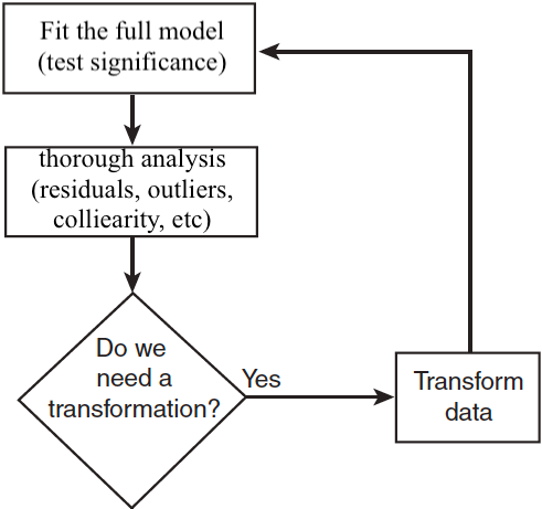
Model Building Process

Model Selection Criteria

Selection Methods

Model Building

So far, we assume that we

• have a very good idea of the basic form of the model (linear form after transformation)
• know (nearly) all of the regressors that are important and should be used.

Model Adequacy

Model Selection

Our strategy is - Fit the full model - Perform a thorough analysis (residual analysis, outliers, collinearity, etc) - Transformation of response/regressors - Test regressor significance - Perform a thorough analysis

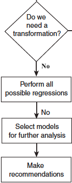
Variable Selection

• We have a large pool of candidate regressors, of which only a few are likely to be important.
• Finding an appropriate subset of regressors for the model is called model/variable selection.

Two “conflicting” goals in model building:

• as many regressors as possible for better predictive performance on new data (smaller bias).

• as few regressors as possible because as the number of regressors increases,

  • \(\mathrm{Var}(\hat{y})\) will increase (larger variance)
  • cost more in data collecting and maintaining
  • more model complexity

A compromise between the two hopefully leads to the “best” regression equation.

What does best mean?

• In most practical problems, we have a large pool of possible candidate regressors, of which only a few are likely to be important.
• Finding an appropriate subset of regressors for the model is called variable selection.
• Two “conflicting” goals in model building:
  • as many regressors as possible for more information for prediction
  • as few regressors as possible (1) the variance of \(\hat{y}\) will increase as the number of regressors increases (2) cost more in data collection (3) more model complexity

A compromise between the two hopefully leads to the “best” regression equation.

There is no unique definition of “best”, and different methods specify different subsets of the candidate regressors as best.

Predictive Performance

• A selected model that fits the observed sample data well may not predict well on new observations.
• Build a good regression function/model in terms of prediction accuracy. (Model validation/assessment)
• Want: The selected model minimizes the mean square prediction error (MSPE) on the new data: \[\small MSPE(\hat{y}) = E\left[ (\hat{y} - y)^2\right] = E\left[ (\hat{y} - E(\hat{y}))^2\right] + [E(\hat{y}) - y]^2 = \mathrm{Var}(\hat{y}) + \text{Bias}^2(\hat{y})\]

• The mechanics of prediction is easy:
  • Plug in values of predictors to the model equation.
  • Calculate the predicted value of the response \(\hat{y}\)

• So, the mechanics of prediction is easy:
  • Once you have your model, you can Plug in values of predictors to the model equation
  • Calculate the predicted value of the response variable, \(\hat{y}\), either numerical or categorical.

• Getting it right is hard! No guarantee that
  • the model estimates are close to the truth
  • your model performs as well with new data as it did with your sample data

• But Getting it right is hard!
  • There is no guarantee the model estimates you have are correct
  • Or that your model will perform as well with new data as it did with your sample data
• Test data are the new data that are not used for training or fitting our model, but the data we are interested in predicting its value.
• So we care about the prediction performance on the test data much more than the performance on the training data.

Spending Our Data

• Several steps to create a useful model:
  • Parameter estimation
  • Model building and selection
  • Performance assessment, etc.

• Doing all of this on the entire data may lead to overfitting:

The model performs well on the current sample data, but awfully predicts the response on the new data we are interested.

• When we are doing modeling, we are doing several steps to create a useful model,
  • parameter estimation
  • model selection
  • performance assessment, etc.
• Doing all of this on the entire data we have available may lead to overfitting. In classification, it means that our model labels the training response variable almost perfectly with very high classification accuracy, but the model performs very bad when fitted to the test data or incoming future emails for example.

Overfitting

The model performs well on the current sample data, but awfully predicts the response on the new data we are interested.

• Low error rate on observed data, but high prediction error rate on future unobserved data!

Source: https://i.pinimg.com/originals/72/e2/22/72e222c1542539754df1d914cb671bd7.png

https://i.pinimg.com/originals/72/e2/22/72e222c1542539754df1d914cb671bd7.png - Look at this illustration, and let’s focus on the overfitting and classification case. - the blue and red points are our training data representing two categories, and the green points are the new data to be classified. - the black curve is the classification boundary that separates the two categories. - Based on the boundary, you can see that the classification performance on the training data set is perfect, because all blue points and red points are perfectly separated. - However, such classification rule generated by the training data may not be good for the new data. - With this boundary, … - OK so, if we wanna make sure that our model is good at predicting things, we probably want to avoid overfitting. - But how?

Splitting Data

• Often, we don’t have another unused data to assess the performance of our model.

• Solution: Pretend we have new data by splitting our data into training set and test set (validation set)!

• Training set:
  • Sandbox for model building/selection
  • Spend most of your time using the training set to develop the model
  • Majority of the original sample data (usually ~ 80%)
• Test set:
  • Held in reserve to determine efficacy of one or two chosen models
  • Critical to look at it once only, otherwise it becomes part of the modeling process
  • Remainder of the data (usually ~ 20%)

• Allocate specific subsets of data for different tasks, as opposed to allocating the largest possible amount to the model parameter estimation only (what we’ve done so far).
• Well we do this by splitting our data. So we split our data into to sets, training set and testing set, or sometimes called validation set.
• You can think about your training set as your sandbox for model building. You can do whatever you want, like data wrangling, data transformation, data tidying, and data visualization, all of which help you build an appropriate model.
• So you Spend most of your time using the training set to develop the model
• And this is the Majority of the original sample data, which is usually about 75% - 80% of your data. So you basically take a random sample from the data that is about 80% of it.
• And you don’t touch the remaining 20% of the data until you are ready to test your model performance.
• So the test set is held in reserve to determine efficacy of one or two chosen models
• Critical to look at it once, otherwise it becomes part of the modeling process
• and that is the Remainder of the data, usually 20% - 25%
• So ideally, we hope to use our entire data as training data to train our model, right? And to test the model performance, we just collect another data set as test data to be used for testing performance. But in reality, it is not the usual case. In reality, we only have one single data set, and it is hard to collect another sample data as test data.
• So under this situation, this type of splitting data becomes a must if we want to have both training and test data.

Model Selection Criteria

• The full (largest) model has \(M\) candidate regressors.

• There are \(M \choose p-1\) possible subset models of size \(p\).

• There are totally \(2^M\) possible subset models.

• An evaluation metric should consider Goodness of Fit and Model Complexity:

Goodness of Fit: The more regressors, the better

Complexity Penalty: The less regressors, the better

• Evaluate subset models:
  • \(R_{adj}^2\) \(\uparrow\)
  • Mallow’s \(C_p\) \(\downarrow\)
  • Information Criterion (AIC, BIC) \(\downarrow\)
  • PREdiction Sum of Squares (PRESS) \(\downarrow\) (Allen, D.M. (1974))

• \(R^2\) \(\uparrow\)
• \(MS_{res}\) \(\downarrow\)
• The idea of model selection is to apply some penalty on the number of parameters used in the model. On one hand, we want to model fitting to be as good as possible, i.e., the mean squared error is small. On the other hand, we also want to restrict on the number of variables. We know that as we keep adding variables into a linear regression, the R2 would usually increase. Hence, there is a trade-off between the two. In general, we consider a criterion in the form of

Selection Criteria: Mallow’s \(C_p\) Statistic \(\downarrow\)

For a model with \(p\) coefficients ( \(k\) predictors ),

\[\begin{align} C_p &= \frac{SS_{res}(p)}{\hat{\sigma}^2} - n + 2p \\ &= p + \frac{(s^2 - \hat{\sigma}^2)(n-p)}{\hat{\sigma}^2} \end{align}\]

• \(\hat{\sigma}^2\) is the variance estimate from the full model, i.e., \(\hat{\sigma}^2 = MS_{res}(M)\).

• \(s^2\) is the variance estimate from the model with \(p\) coefficients, i.e., \(s^2 = MS_{res}(p)\).

• Favors the candidate model with the smallest \(C_p\).

• For unbiased models that \(E[\hat{y}_i] = E[y_i]\), \(C_p = p\).

  • All of the errors in \(\hat{y}_i\) is variance, and the model is not underfitted.

• \(C_p = M + 1\) for the full model.

Mallow’s \(C_p\) Plot

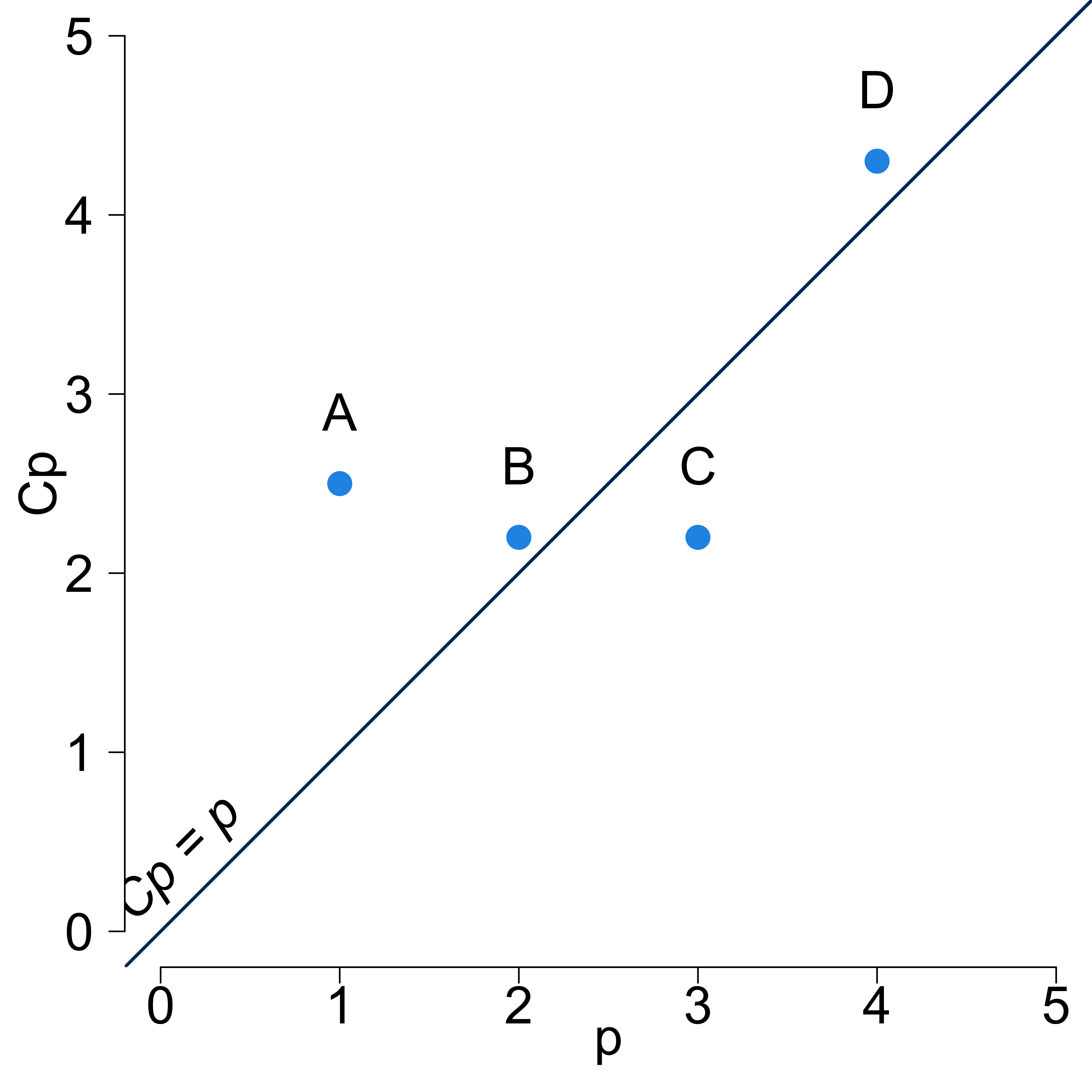
• Model A is a heavily biased model.
• Model D is the poorest performer.
• Model B and C are reasonable.
• Model C has \(C_p < 3\) which implies \(MS_{res}(3) < MS_{res}(M)\)

Selection Criteria: Information Criterion \(\downarrow\)

For a model with \(p\) coefficients ( \(k\) predictors ),

• Akaike information criterion (AIC) is \[\text{AIC} = n \ln \left( \frac{SS_{res}(p)}{n} \right) + 2p\]
• Bayesian information criterion (BIC) is \[\text{BIC} = n \ln \left( \frac{SS_{res}(p)}{n} \right) + p \ln (n)\]
• BIC penalizes more when adding more variables as the sample size increases.
• BIC tends to choose models with less regressors.

Selection Criteria: PRESS \(\downarrow\)

• Predicted Residual Error Sum of Squares (PRESS)

• \(\text{PRESS}_p = \sum_{i=1}^n[y_i - \hat{y}_{(i)}]^2 = \sum_{i=1}^n\left( \frac{e_i}{1-h_{ii}}\right)^2\) where \(e_i = y_i - \hat{y}_i\).

• \(R_{pred, p}^2 = 1 - \frac{PRESS_p}{SS_T}\)

• \(\text{Absolute PRESS}_p = \sum_{i=1}^n|y_i - \hat{y}_{(i)}|\) can also be considered when some large prediction errors are too influential.

R Lab Criteria Computation

manpower <- read.csv(file = "./data/manpower.csv", header = TRUE)
lm_full <- lm(y ~ x1 + x2 + x3 + x4 + x5, 
              data = manpower)
summ_full <- summary(lm_full)

## Adjusted R sq.
summ_full$adj.r.squared  

[1] 0.987

# PRESS
sum((lm_full$residual / 
       (1 - hatvalues(lm_full))) ^ 2) 

[1] 32195222

• ols_mallows_cp() for Mallow’s \(C_p\) in olsrr package

## AIC
extractAIC(lm_full, k = 2)  

[1]   6 224

## BIC
n <- length(manpower$y)
extractAIC(lm_full, k = log(n)) 

[1]   6 229

'log Lik.' -130 (df=7)

[1] 224

[1] 229

[1] 4.43

Selection Methods: Best Subset (All Possible) Selection

• Assume the intercept is in all models.
• If there are \(M\) possible regressors, we investigate all \(2^M - 1\) possible regression equations.
• Use the selection criteria to determine some candidate models and complete regression analysis on them.
• If the estimates of a particular coefficient tends to “jump around”, this could be an indication of collinearity.

R Lab Best Subset Selection ols_step_all_possible()

olsrr_all <- olsrr::ols_step_all_possible(lm_full)
names(olsrr_all)

 [1] "mindex"     "n"          "predictors" "rsquare"    "adjr"      
 [6] "predrsq"    "cp"         "aic"        "sbic"       "sbc"       
[11] "msep"       "fpe"        "apc"        "hsp"       

• n: number of predictors
• predictors: predictors in the model
• rsquare: R-square of the model
• adjr: adjusted R-square of the model
• predrsq: predicted R-square of the model

• cp: Mallow’s Cp
• aic: AIC
• sbic: Sawa BIC
• sbc: Schwarz BIC (the one we defined)

Model (x2 x3 x5)

   Index N     Predictors R-Square Adj. R-Square Mallow's Cp
3      1 1             x3    0.972         0.970       20.38
1      2 1             x1    0.971         0.970       21.20
2      3 1             x2    0.893         0.886      114.97
4      4 1             x4    0.884         0.877      125.87
5      5 1             x5    0.335         0.290      785.26
10     6 2          x2 x3    0.987         0.985        4.94
6      7 2          x1 x2    0.986         0.984        5.66
14     8 2          x3 x5    0.985         0.983        7.29
9      9 2          x1 x5    0.984         0.982        8.16
13    10 2          x3 x4    0.975         0.972       18.57
8     11 2          x1 x4    0.974         0.970       20.04
7     12 2          x1 x3    0.973         0.969       21.99
11    13 2          x2 x4    0.931         0.921       72.29
12    14 2          x2 x5    0.924         0.913       80.30
15    15 2          x4 x5    0.910         0.898       96.50
23    16 3       x2 x3 x5    0.990         0.988        2.92
18    17 3       x1 x2 x5    0.989         0.987        3.71
16    18 3       x1 x2 x3    0.987         0.984        6.21
22    19 3       x2 x3 x4    0.987         0.984        6.90
17    20 3       x1 x2 x4    0.986         0.983        7.66
20    21 3       x1 x3 x5    0.985         0.982        8.97
25    22 3       x3 x4 x5    0.985         0.982        9.00
21    23 3       x1 x4 x5    0.985         0.981        9.41
19    24 3       x1 x3 x4    0.978         0.974       16.80
24    25 3       x2 x4 x5    0.952         0.941       48.28
30    26 4    x2 x3 x4 x5    0.991         0.988        4.03
28    27 4    x1 x2 x4 x5    0.991         0.987        4.26
27    28 4    x1 x2 x3 x5    0.991         0.987        4.35
26    29 4    x1 x2 x3 x4    0.988         0.984        7.54
29    30 4    x1 x3 x4 x5    0.985         0.980       10.92
31    31 5 x1 x2 x3 x4 x5    0.991         0.987        6.00

[1] 275

[1] 273

[1] 224

[1] 280

[1] 278

[1] 229

[1] 278

[1] 280

[1] 232

R Lab ols_step_best_subset()

# metric = c("rsquare", "adjr", "predrsq", "cp", "aic", "sbic", "sbc", "msep", "fpe", "apc", "hsp")
olsrr::ols_step_best_subset(lm_full, metric = "predrsq")

   Best Subsets Regression   
-----------------------------
Model Index    Predictors
-----------------------------
     1         x3             
     2         x2 x3          
     3         x2 x3 x5       
     4         x2 x3 x4 x5    
     5         x1 x2 x3 x4 x5 
-----------------------------

                                                           Subsets Regression Summary                                                            
-------------------------------------------------------------------------------------------------------------------------------------------------
                       Adj.        Pred                                                                                                           
Model    R-Square    R-Square    R-Square     C(p)        AIC         SBIC        SBC           MSEP             FPE            HSP         APC  
-------------------------------------------------------------------------------------------------------------------------------------------------
  1        0.9722      0.9703       0.956    20.3812    285.5158    234.8274    288.0155    15612703.3319    1025426.9349    65534.8041    0.0352 
  2        0.9867      0.9848       0.964     4.9416    274.9519    227.0975    278.2847     8029607.6257     552301.0536    36111.9920    0.0190 
  3        0.9901      0.9878       0.964     2.9177    272.0064    226.8104    276.1724     6503027.4301     466884.0206    31496.1442    0.0160 
  4        0.9908      0.9877       0.942     4.0263    272.6849    229.2716    277.6841     6563621.8068     490245.8263    34438.7564    0.0168 
  5        0.9908      0.9867       0.935     6.0000    274.6442    232.3507    280.4767     7202730.2305     557787.1896    41227.7488    0.0192 
-------------------------------------------------------------------------------------------------------------------------------------------------
AIC: Akaike Information Criteria 
 SBIC: Sawa's Bayesian Information Criteria 
 SBC: Schwarz Bayesian Criteria 
 MSEP: Estimated error of prediction, assuming multivariate normality 
 FPE: Final Prediction Error 
 HSP: Hocking's Sp 
 APC: Amemiya Prediction Criteria 

• ols_step_best_subset() identifies the best model of each size using \(R^2\) by default.

R Lab Best Subset Selection

k	1	2	3	4	5	r2	adj_r2	cp	press	abs_press	r2_pred	aic	bic
1	0	0	1	0	0	0.972	0.970	20.38	2.18e+07	13431	0.956	235	237
1	1	0	0	0	0	0.971	0.970	21.20	2.22e+07	13666	0.955	236	237
1	0	1	0	0	0	0.893	0.886	114.97	1.58e+08	28031	0.680	258	260
1	0	0	0	1	0	0.884	0.877	125.87	7.01e+07	22890	0.858	260	261
1	0	0	0	0	1	0.335	0.290	785.26	4.56e+08	61324	0.079	289	291
2	0	1	1	0	0	0.987	0.985	4.94	1.79e+07	12742	0.964	225	227
2	1	1	0	0	0	0.986	0.984	5.66	1.80e+07	12873	0.964	225	228
2	0	0	1	0	1	0.985	0.983	7.29	1.26e+07	10915	0.974	227	230
2	1	0	0	0	1	0.984	0.982	8.16	1.30e+07	11074	0.974	228	230
2	0	0	1	1	0	0.975	0.972	18.57	3.25e+07	16825	0.934	235	238
2	1	0	0	1	0	0.974	0.970	20.04	3.58e+07	17328	0.928	236	239
2	1	0	1	0	0	0.973	0.969	21.99	2.26e+07	13957	0.954	237	240
2	0	1	0	1	0	0.931	0.921	72.29	1.41e+08	28166	0.716	253	255
2	0	1	0	0	1	0.924	0.913	80.30	1.29e+08	25960	0.740	254	257
2	0	0	0	1	1	0.910	0.898	96.50	7.12e+07	25251	0.856	257	260

k	1	2	3	4	5	r2	adj_r2	cp	press	abs_press	r2_pred	aic	bic
3	0	1	1	0	1	0.990	0.988	2.92	1.78e+07	12019	0.964	222	225
3	1	1	0	0	1	0.989	0.987	3.71	1.81e+07	12163	0.964	223	226
3	1	1	1	0	0	0.987	0.984	6.21	2.28e+07	14243	0.954	226	229
3	0	1	1	1	0	0.987	0.984	6.90	3.01e+07	15780	0.939	227	230
3	1	1	0	1	0	0.986	0.983	7.66	3.28e+07	16227	0.934	227	231
3	1	0	1	0	1	0.985	0.982	8.97	1.30e+07	11104	0.974	229	232
3	0	0	1	1	1	0.985	0.982	9.00	1.63e+07	11801	0.967	229	232
3	1	0	0	1	1	0.985	0.981	9.41	1.78e+07	12296	0.964	229	232
3	1	0	1	1	0	0.978	0.974	16.80	3.44e+07	18046	0.930	235	238
3	0	1	0	1	1	0.952	0.941	48.28	1.07e+08	26242	0.784	248	252
4	0	1	1	1	1	0.991	0.988	4.03	2.86e+07	14606	0.942	222	227
4	1	1	0	1	1	0.991	0.987	4.26	3.03e+07	14992	0.939	223	227
4	1	1	1	0	1	0.991	0.987	4.35	2.25e+07	13364	0.955	223	227
4	1	1	1	1	0	0.988	0.984	7.54	3.77e+07	17952	0.924	227	231
4	1	0	1	1	1	0.985	0.980	10.92	1.86e+07	12773	0.962	231	235
5	1	1	1	1	1	0.991	0.987	6.00	3.22e+07	16025	0.935	224	229

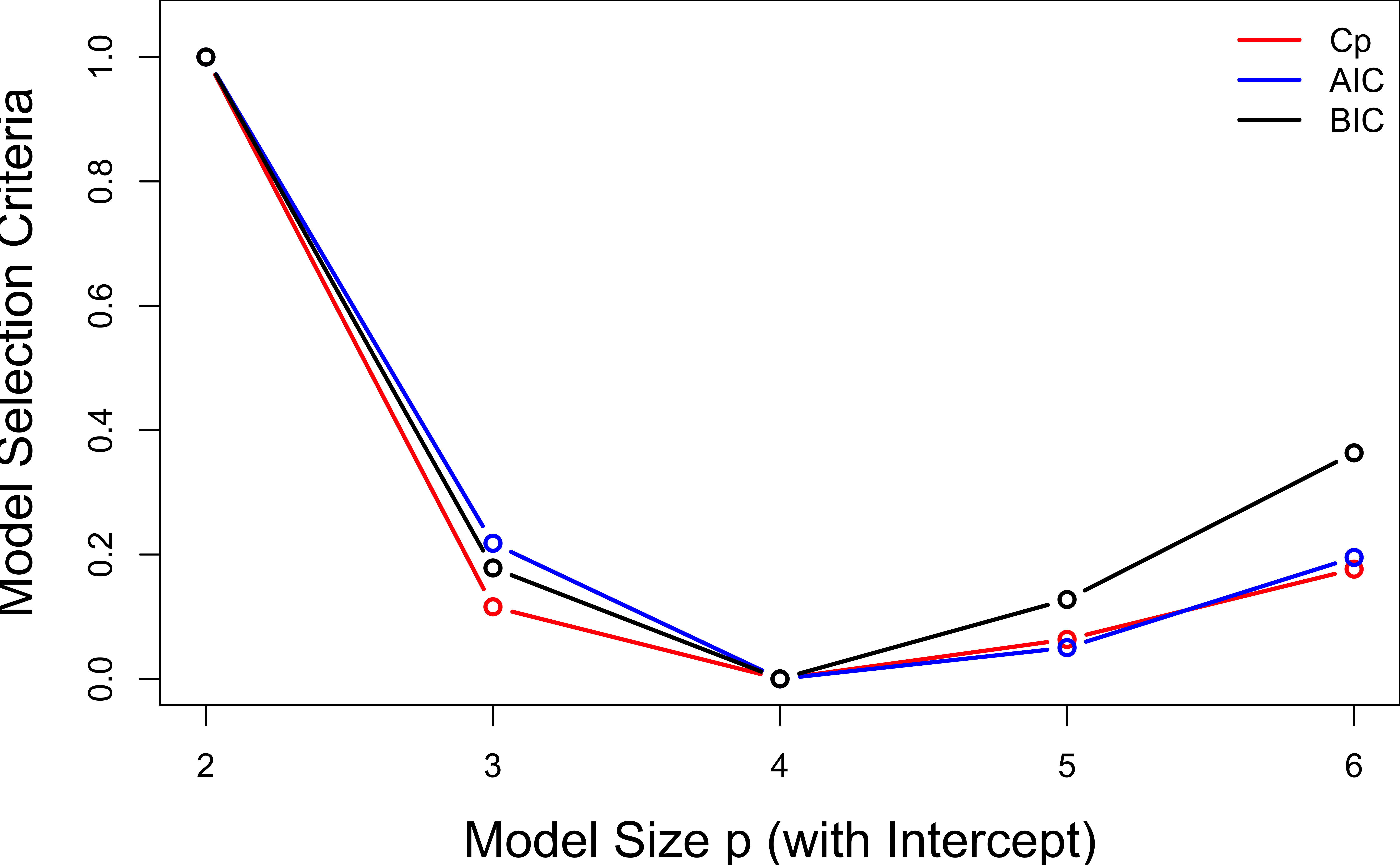
R Lab Best Subset Selection

Scale Cp, AIC, BIC to \([0, 1]\).

Selection Methods: Forward Selection

• Begins with no regressors.
• Insert regressors into the model one at a time.

• The first regressor selected, \(x_1\), is the one producing the largest \(R^2\) of any single regressor. It is the one with
  • the highest correlation with the response.
  • the largest \(F_{test}\) and \(F_{test} > F_{IN}(\alpha, 1, n-2)\), where \(F_{IN}\) is the pre-specified \(F\) threshold.

• The second regressor \(x_2\) produces the largest increase in \(R^2\) in the presence of \(x_1\). It is the one with
  • the largest partial correlation with the response.
  • the largest partial \(F_{test} = \frac{SS_R(x_2|x_1)}{MS_{res}(x_1, x_2)}\) and \(F_{test} > F_{IN}(\alpha, 1, n-3)\)

• The process terminates when
  • partial \(F_{test} <F_{IN}(\alpha, 1, n-p)\), or
  • the last candidate regressor is added to the model.

\(F_{test} > F_{\alpha, 1, n-2}\) \(F_{test} = \frac{SS_R(x_2|x_1)}{MS_{res}(x_1, x_2)}> F_{\alpha, 1, n-2}\) Once a regressor has been added, it cannot be removed at a later step. - Begins with no regressors in the model other than the intercept. - Insert regressors into the model one at a time. - The first regressor selected to be entered into the model, say \(x_1\), is the one that produces the largest \(R^2\) of any single regressor. + the one with the highest correlation with the response. + the one with the largest \(F_{test}\) and \(F_{test} > F_{IN}\) - The second regressor examined is the one, say \(x_2\), that produces the largest increase in \(R^2\) in the presence of \(x_1\). + the one with the largest partial correlation with the response. + the one with the largest \(F_{test} = \frac{SS_R(x_2|x_1)}{MS_{res}(x_1, x_2)}\) and \(F_{test} > F_{IN}\) - The process terminates either when the partial \(F\) statistic at a particular step does not exceed \(F_{IN}\) or when the last candidate regressor is added to the model.

R Lab Forward Selection ols_step_forward_p()

• The default threshold compared with the \(p\)-value \(=P(F_{1, n-p} > F_{test})\) is 0.3.
• If \(p\)-value < 0.3, the regressor is entered.

(olsrr_for <- olsrr::ols_step_forward_p(lm_full, penter = 0.3))

                             Selection Summary                              
---------------------------------------------------------------------------
        Variable                  Adj.                                         
Step    Entered     R-Square    R-Square     C(p)        AIC         RMSE      
---------------------------------------------------------------------------
   1    x3            0.9722      0.9703    20.3812    285.5158    957.8556    
   2    x2            0.9867      0.9848     4.9416    274.9519    685.1685    
   3    x5            0.9901      0.9878     2.9177    272.0064    614.7794    
---------------------------------------------------------------------------

# names(olsrr_for)

R Lab Forward Selection ols_step_forward_p()

olsrr_for$model

Call:
lm(formula = paste(response, "~", paste(preds, collapse = " + ")), 
    data = l)

Coefficients:
(Intercept)           x3           x2           x5  
   1523.389        0.978        0.053     -320.951  

• progress = TRUE, details = TRUE for detailed selection progress.

olsrr::ols_step_forward_p(lm_full, penter = 0.3, progress = TRUE, details = TRUE)

Selection Methods: Stepwise Regression

• This procedure is a modification of forward selection.
• At each step, all regressors put into the model are reassessed via their partial \(F\) statistic.
• A regressor added at an earlier step may now be redundant because of the relationships between it and regressors now in the equation.
• If the partial \(F_{test} < F_{OUT}\), the variable will be removed.
• The method requires both an \(F_{IN}\) and \(F_{OUT}\).

it becomes insignificant with the addition of other variables to the model.

R Lab Stepwise Regression ols_step_both_p()

• If \(p\)-value < pent = 0.1, the regressor is entered.
• After refitting, the regressor is removed if \(p\)-value > prem = 0.3.

(olsrr_both <- olsrr::ols_step_both_p(lm_full, pent = 0.1, prem = 0.3))

                              Stepwise Selection Summary                                
---------------------------------------------------------------------------------------
                     Added/                   Adj.                                         
Step    Variable    Removed     R-Square    R-Square     C(p)        AIC         RMSE      
---------------------------------------------------------------------------------------
   1       x3       addition       0.972       0.970    20.3810    285.5158    957.8556    
   2       x2       addition       0.987       0.985     4.9420    274.9519    685.1685    
   3       x5       addition       0.990       0.988     2.9180    272.0064    614.7794    
---------------------------------------------------------------------------------------

Comments on Stepwise-Type Procedures

• There is a backward elimination stepwise-type procedure
  • Begin with the model with all \(M\) candidate regressors.
  • Remove regressors from the model one at a time.
  • olsrr::ols_step_backward_p()
  • Check Variable Selection Methods

• One can select models/variables based on other metrics such as AIC
  • olsrr::ols_step_forward_aic()
  • olsrr::ols_step_both_aic()
  • olsrr::ols_step_backward_aic()

• The order in which the regressors enter or leave the model does not imply an order of importance to the regressors.

• No one model may be the “best”.

• Different stepwise techniques could result in different models.

• The order in which the regressors enter or leave the model does not imply an order of importance to the regressors.
• This is in fact a general problem with the forward selection procedure. Once a regressor has been added, it cannot be removed at a later step.
• forward selection tends to agree with all possible regressions for small subset sizes but not for large ones
• backward elimination tends to agree with all possible regressions for large subset sizes but not for small ones.
• the most common being that none of the procedures generally guarantees that the best subset regression model of any size will be identified.
• there is one best subset model, but that there are several equally good ones.

set F IN = F OUT = 4, as this corresponds roughly to the upper 5% point of the F distribution Bendel and Afi fi [ 1974 ] recommend α = 0.25 for forward selection. F IN of between 1.3 and 2.

Kennedy and Bancroft [ 1971] suggest α = 0.25 for forward selection and recommend α = 0.10 for backward elimi

• STRATEGY FOR VARIABLE SELECTION AND MODEL BUILDING the PRESS statistic tends to recommend smaller models than Mallow’s Cp, which in turn tends to recommend smaller models than the adjusted R2 .