Nonparametric Regression 🛠

MATH 4780 / MSSC 5780 Regression Analysis

Dr. Cheng-Han Yu
Department of Mathematical and Statistical Sciences
Marquette University

Nonparametric Regression

Nonparametric Kernel Smoother

Local Regression

Nonparametric Statistics

• A general regression model \(y = f(x) + \epsilon\).
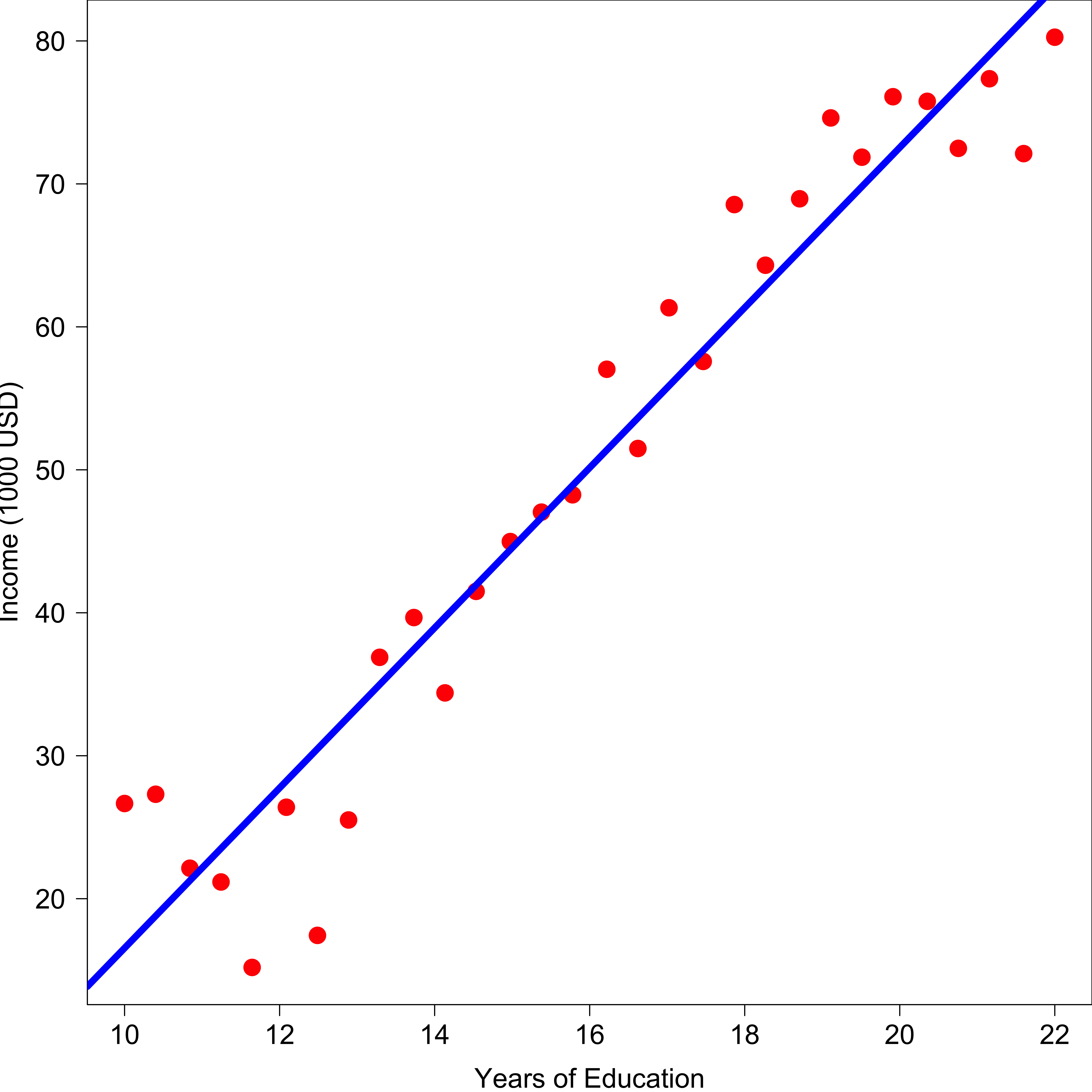
• Parametric model: make an assumption about the shape of \(f\), e.g., \(f(x) = \beta_0 + \beta_1 x\), then learn the parameters \(\beta_0\) and \(\beta_1\).

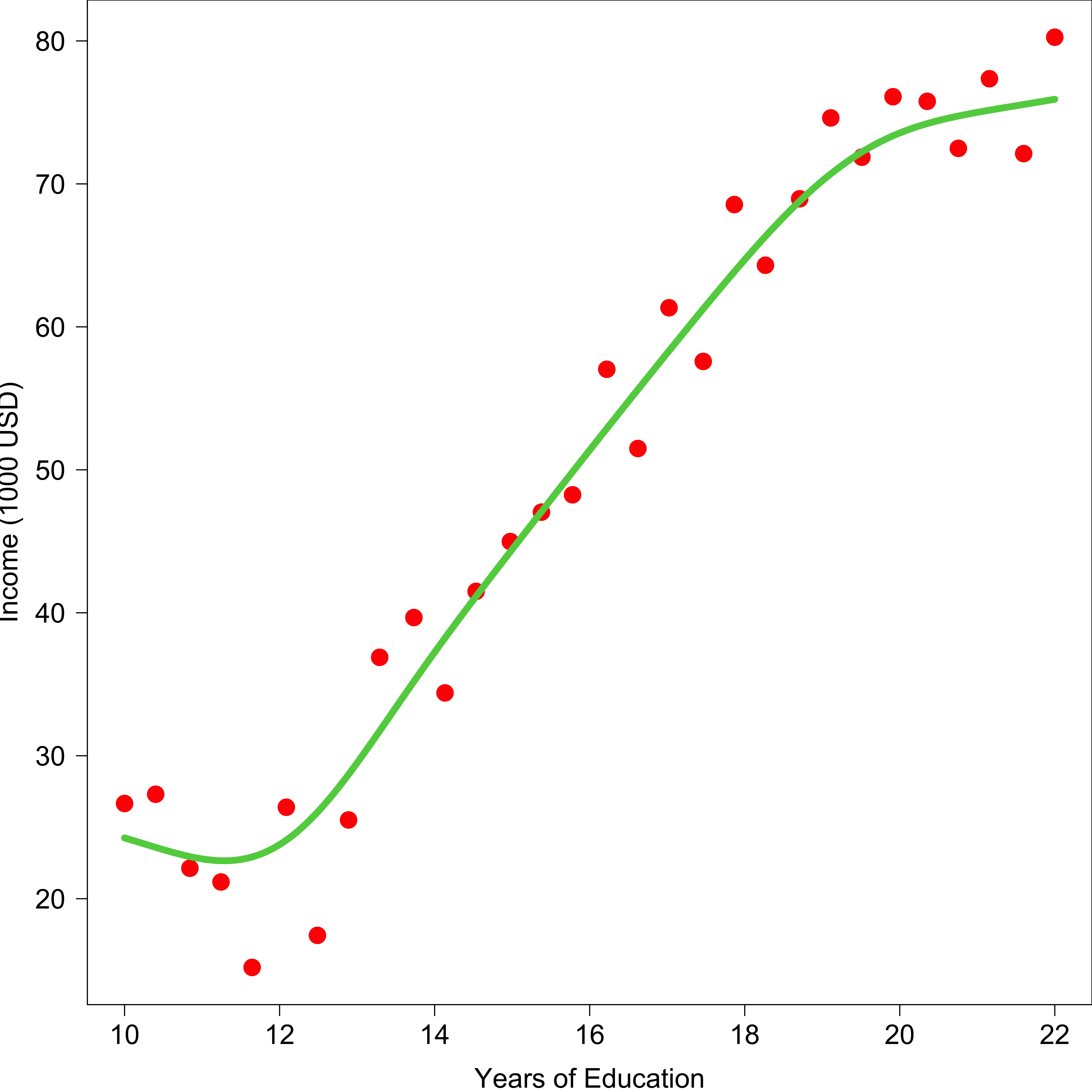
• Nonparametric methods do NOT make assumptions about the form of \(f\).
  • Seek an estimate of \(f\) that gets close to the data points without being too rough or wiggly.
  • Avoid the possibility that the functional form used to estimate \(f\) is very different from the true \(f\).
  • Do not reduce the problem of estimating \(f\) to a small number of parameters, so more data are required to obtain an accurate estimate of \(f\).

• So far, with a general regression model \(y = f(x) + \epsilon\), we make an assumption about the form or shape of \(f\), for example, \(f(x) = \beta_0 + \beta_1 x\), then learn the parameters \(\beta_0\) and \(\beta_1\) to understand the relationship between \(y\) and \(x\). This is a parametric model.
• Nonparametric methods do not make assumptions about the form of \(f\).
  • They seek an estimate of \(f\) that gets close to the data points without being too rough or wiggly.
  • The methods avoid the possibility that the functional form used to estimate \(f\) is very different from the true \(f\).
  • Since they do not reduce the problem of estimating \(f\) to a small number of parameters, more observations are required to obtain an accurate estimate for \(f\).

Parametric vs. Nonparametric Models

Parametric (Linear regression)

Nonparametric (Kernel smoother)

Nonparametric Regression

• In (parametric) linear regression, \(\small \hat{y}_i = \sum_{j=1}^n h_{ij}y_j\).
• Nonparametric regression, with no assumption on \(f\), is trying to estimate \(y_i\) using the weighted average of the data: \[\small \hat{y}_i = \sum_{j=1}^n w_{ij}y_j\] where \(\sum_{j=1}^nw_{ij} = 1\).

\(w_{ij}\) is larger when \(x_i\) and \(x_j\) are closer. \(y_i\) is affected more by its neighbors.

\[\small {\bf \hat{y} = Xb = X(X'X)^{-1}X'y = Hy},\] - \(w_{ij}\): the influence power of \(y_j\) on \(y_i\).

Kernel Smoother

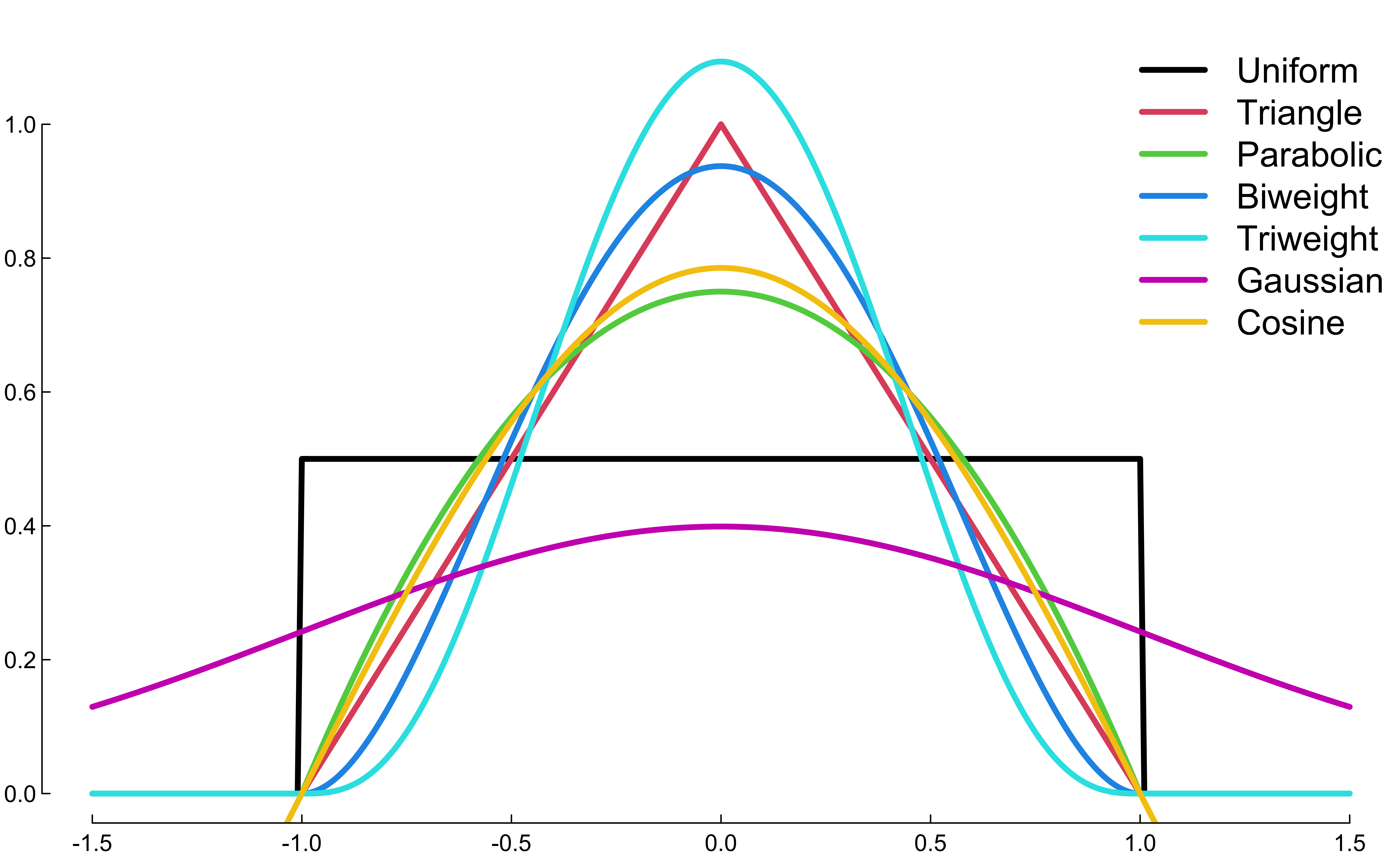
• In nonparametric statistics, a kernel \(K(t)\) is used as a weighting function satisfying
  • \(K(t) \ge 0\) for all \(t\)
  • \(\int_{-\infty}^{\infty} K(t) \,dt = 1\)
  • \(K(-t) = K(t)\) for all \(t\)

Can you give me an kernel function?

Kernel Smoother

• In nonparametric statistics, a kernel \(K(t)\) is used as a weighting function satisfying
  • \(K(t) \ge 0\) for all \(t\)
  • \(\int_{-\infty}^{\infty} K(t) \,dt = 1\)
  • \(K(-t) = K(t)\) for all \(t\)

Kernel Smoother

• Let \(\tilde{y}_i\) be the kernel smoother of the \(i\)th response. Then \[\small \tilde{y}_i = \sum_{j=1}^n w_{ij}y_j\] where \(\sum_{j=1}^nw_{ij} = 1\).

• The Nadaraya–Watson kernel regression uses the weights given by \[\small w_{ij} = \frac{K \left( \frac{x_i - x_j}{b}\right)}{\sum_{k=1}^nK \left( \frac{x_i - x_k}{b}\right)}\]

  • Parameter \(b\) is the bandwidth that controls the smoothness of the fitted curve.
  • Closer points are given higher weights: \(w_{ij}\) is larger if \(x_i\) and \(x_j\) are closer.

• \(\tilde{y}_i\)s will not be as much variationed as \(y_j\).
• By weighted averaging, the value \(\tilde{y}_i\) is synthesized or integrated by other data points. The average value tends to wash out some unexplained noises, and look more like its other data points.
• These kernel smoothers use a bandwidth, \(b\), to define this neighborhood of interest.

Gaussian Kernel Smoother Example

ksmooth(x, y, bandwidth = 1, kernel = "normal")
KernSmooth::locpoly(x, y, degree = 0, kernel = "normal", bandwidth = 1)

• \(y = 2\sin(x) + \epsilon\)
• \(K_b(x_i, x_j) = \frac{1}{b \sqrt{2\pi}}\exp \left( - \frac{(x_i - x_j)^2}{2b^2}\right)\)

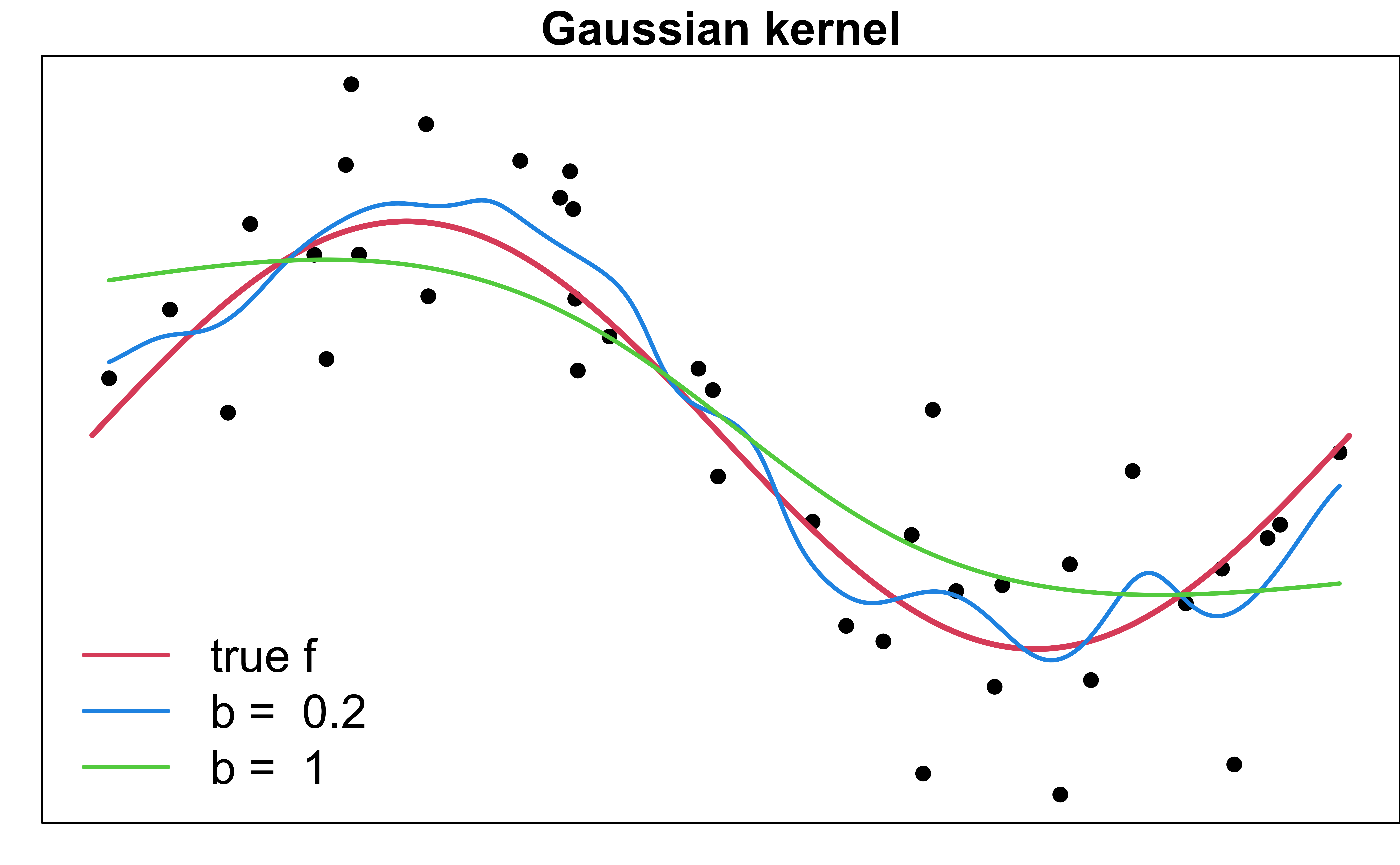
\[\small w_{ij} = \frac{K \left( \frac{x_i - x_j}{b}\right)}{\sum_{k=1}^nK \left( \frac{x_i - x_k}{b}\right)}\] Bandwidth \(b\) defines “neighbors” of \(x_i\), and controls the smoothness of the estimated \(f\).

• Large \(b\): More data points have large weights. The fitted curve becomes smoother
• Small \(b\): Less of the data are used, and the resulting curve looks wiggly.

• Bandwidth \(b\) defines “neighbors” of the specific location of interest, and control the smoothness of the estimated function \(f\).
• When \(b\) is large, more data points with large weights are used to predict the response \(y_i\) at the specific \(x_i\). The fitted curve becomes smoother as \(b\) increases.
• As \(b\) decreases, less of the data are used, and the resulting curve looks more wiggly.
• When \(b\) is large, more points having large weights to predict the response at the specific \(x\). The resulting plot of predicted values becomes smoother as \(b\) increases.
• These kernel smoothers use a bandwidth, \(b\), to define this neighborhood of interest.
• A large value for \(b\) results in more of the data being used to predict the response at the specific location. Consequently, the resulting plot of predicted values becomes much smoother as \(b\) increases.
• Conversely, as \(b\) decreases, less of the data are used to generate the prediction, and the resulting plot looks more “wiggly” or bumpy.

Gaussian Kernel Smoother Example

• The kernel function shows the weights and how fast the weights decay.
• Point sizes correspond to their kernel weight, or the influence on the fitted or predicted value of \(y\) at \(x\).
• To get the estimated fitted curve, we can create a grid of \(x\) points. For each \(x\), find its response value by taking weighted average of the data points whose weight is determined by the kernel function.
• The estimated regression function \(f\) is the result of connecting all the weighted average responses of the \(x\)s in the grid.

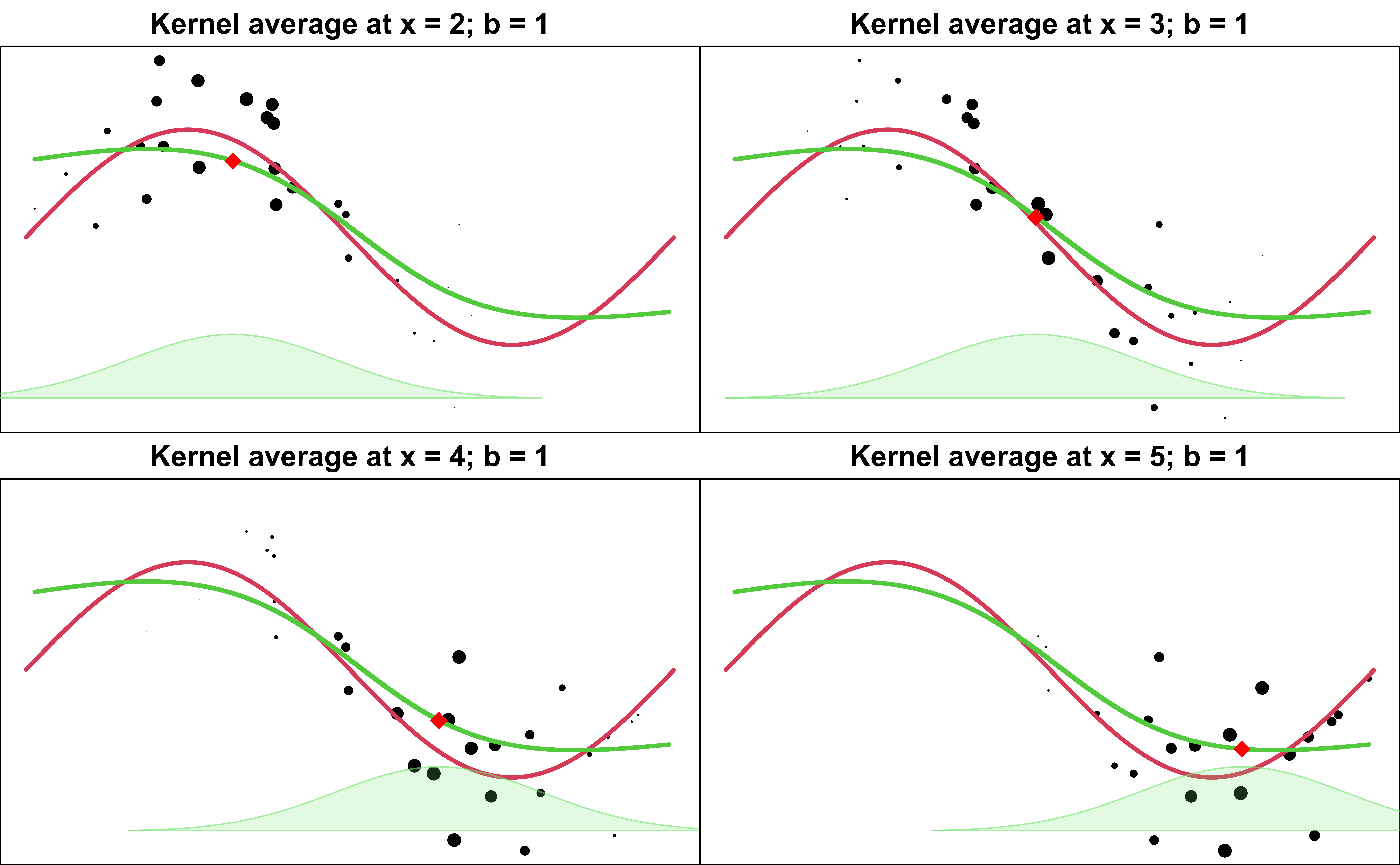
Gaussian Kernel Smoother Example

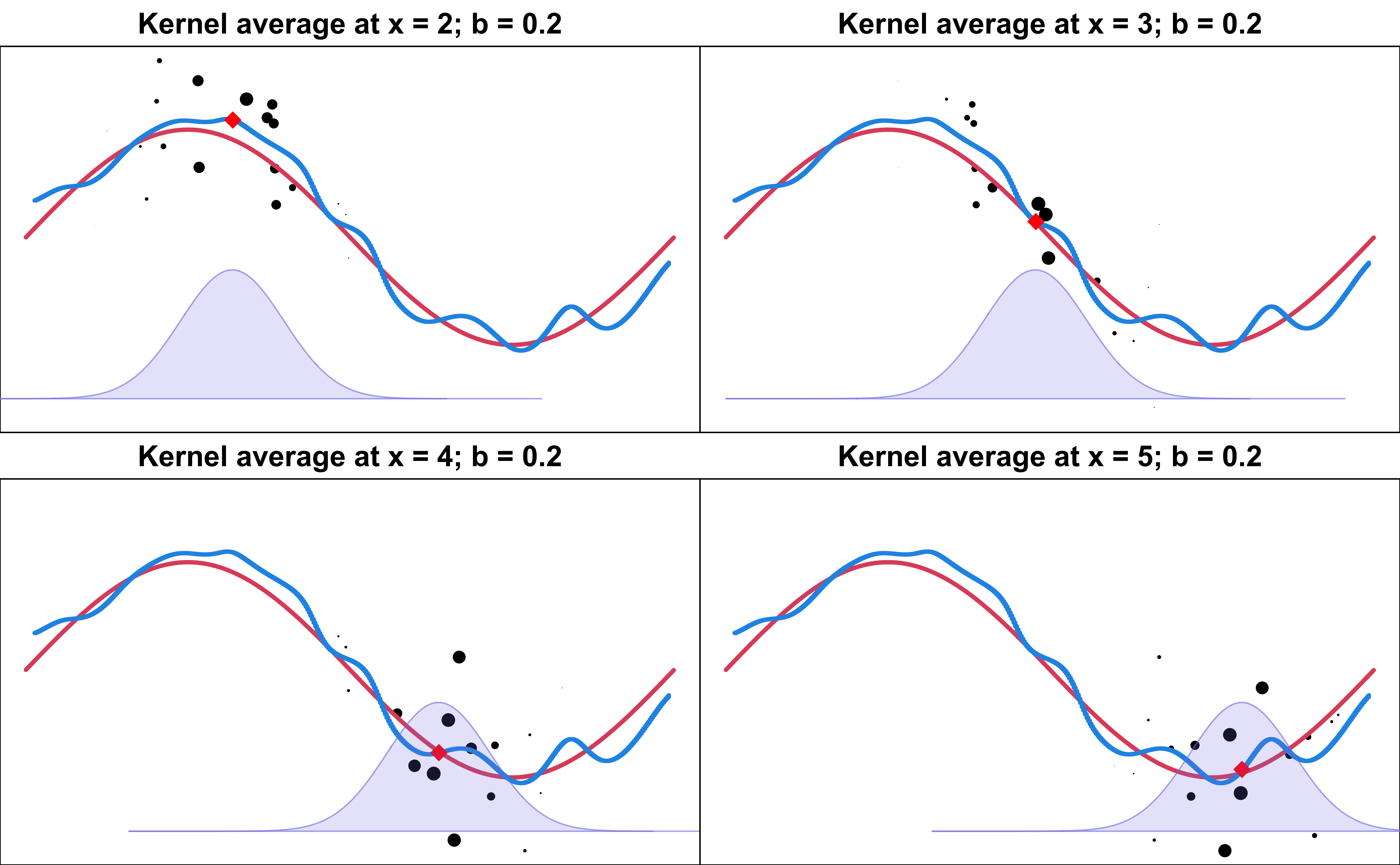
Local Regression

• Local regression is another nonparametric regression alternative.

• In ordinary least squares, minimize \(\sum_{i=1}^n(y_i - \beta_0 - \beta_1x_i)^2\)
• In weighted least squares, minimize \(\sum_{i=1}^nw_i(y_i - \beta_0 - \beta_1x_i)^2\)

In local weighted linear regression,

• Use a kernel as a weighting function to define neighborhoods and weights to perform weighted least squares.

• Find the estimates of \(\beta_0\) and \(\beta_1\) at \(x_0\) by minimizing \[\sum_{i=1}^nK_b(x_0, x_i)(y_i - \beta_0 - \beta_1x_i)^2\]

• Local regression (local polynomial regression, moving regression) is another nonparametric regression alternative.
• Idea: Use a kernel as a weighting function to define neighborhoods and weights to perform weighted least squares.
  • Local weighted linear regression
  • Local weighted polynomial regression

Local Regression

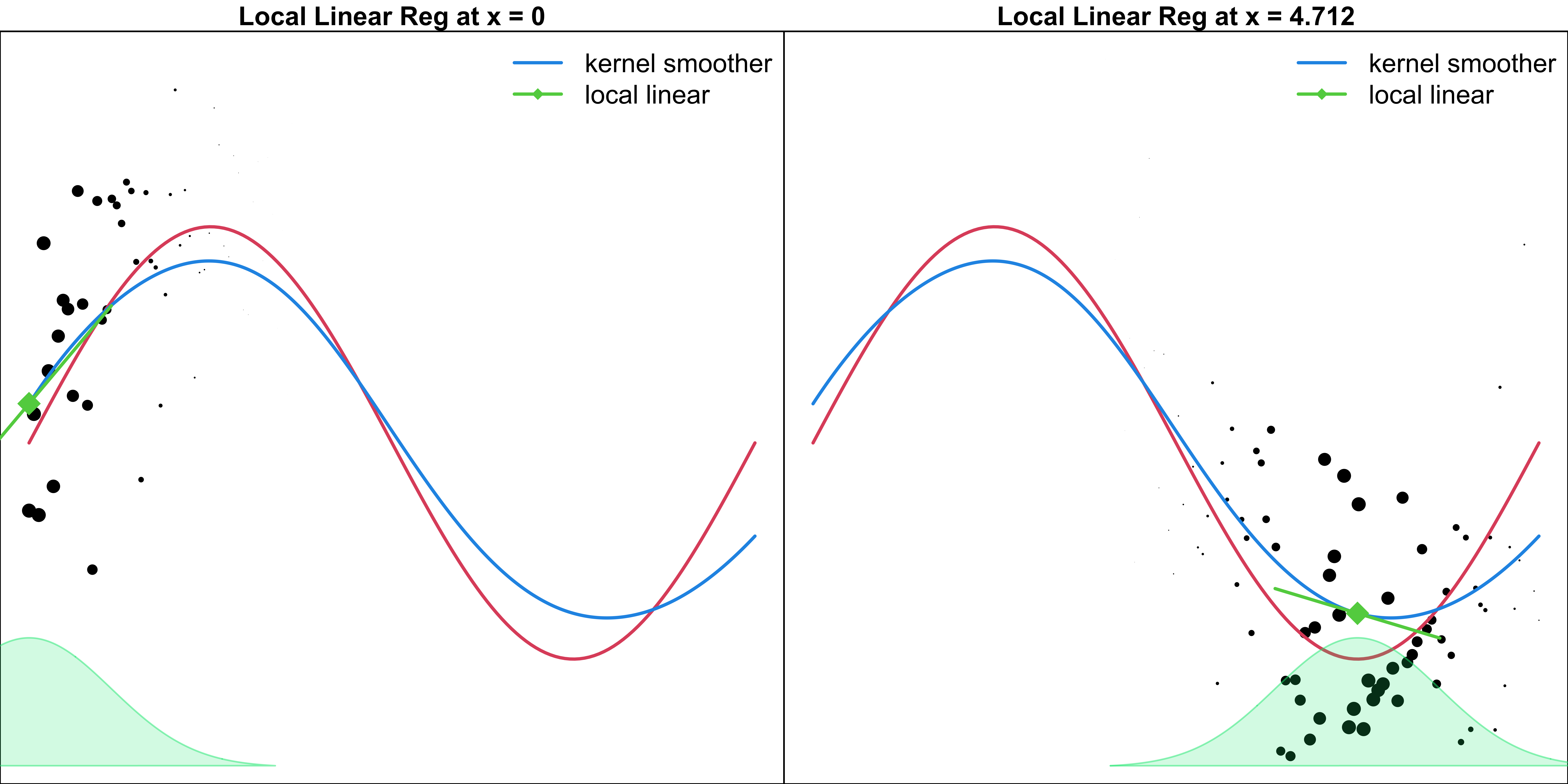
In locally weighted linear regression, we find the estimates of \(\beta_0\) and \(\beta_1\) at \(x_0\) by minimizing \[\sum_{i=1}^nK_b(x_0, x_i)(y_i - \beta_0 - \beta_1x_i)^2\]

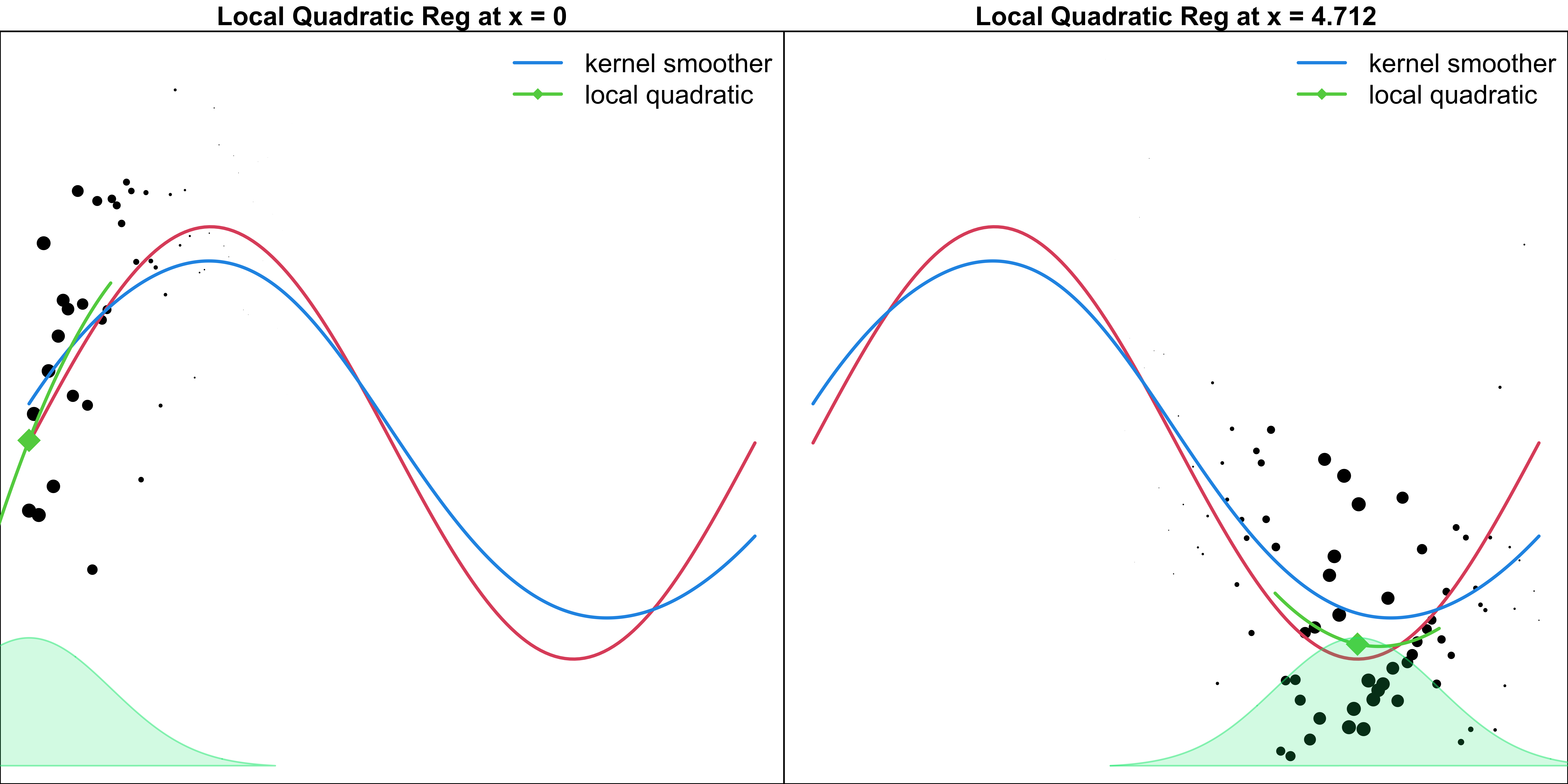
• Pay more attention to the points that are closer to the target point \(x_0\).

• The estimated (local) linear function and \(\hat{\beta}_0\) and \(\hat{\beta}_1\) are only valid at the local point \(x_0\).

• If interested in a different target \(x_0\), we need to refit the model.

• In locally weighted polynomial regression, minimize \[\sum_{i=1}^nK_b(x_0, x_i)(y_i - \beta_0 - \sum_{r=1}^d\beta_rx_i^r)^2\]

• \(\hat{\beta}_0\) and \(\hat{\beta}_1\) are a function of \(x_0\) (of course a function of \((x_i, y_i)_{i=1}^n\)).

Local Linear Regression w/ Gaussian Kernel Weights

Local Quadratic Regression w/ Gaussian Weights

Local Polynomial Regression in R

Use KernSmooth or locfit package.

library(KernSmooth)
locpoly(x, y, degree, 
        kernel = "normal", 
        bandwidth, ...)

• degree = 1: local linear
• degree = 2: local quadratic
• degree = 0: kernel smoother

library(locfit)
locfit(y ~ lp(x, nn = 0.2, 
              h = 0.5, deg = 2), 
       weights = 1, subset, ...)
# weights: Prior weights (or sample sizes) 
#          for individual observations.
# subset: Subset observations in the 
#         data frame.
# nn: Nearest neighbor component of 
#     the smoothing parameter. 
# h: The constant component of 
#    the smoothing parameter.
# deg: Degree of polynomial to use.

• Various ways to specify the bandwidth.

How does local regression determine the weights?

• But why local regression?
  • The Nadaraya-Watson kernel is notorious for boundary effects.
  • There is a substantial bias at the boundaries.
  • Intuition: all neighbors are smaller/larger than the boundary point.
  • Solution: Locally weighted regression can (partially) correct it.
• Its most common methods are LOESS (locally estimated scatterplot smoothing) and LOWESS (locally weighted scatterplot smoothing).
• Like kernel regression, LOESS uses the data from a neighborhood around the specific location.
• The neighborhood \(N(x_0)\) is defined by the span parameter \(\alpha\), the fraction of the total points closest to \(x_0\).
• The LOESS uses the points in \(N(x_0)\) to generate a weighted least-squares estimate of \(y(x_0)\).

LOESS

LOESS (LOcally Estimated Scatterplot Smoothing) uses the tricube kernel \(K(x_0, x_i)\) defined as \[K\left( \frac{|x_0 - x_i|}{\max_{k \in N(x_0)} |x_0 - x_k|}\right)\] where \[K(t) = \begin{cases} (1-t^3)^3 & \quad \text{for } 0 \le t \le 1\\ 0 & \quad \text{otherwise } \end{cases}\]

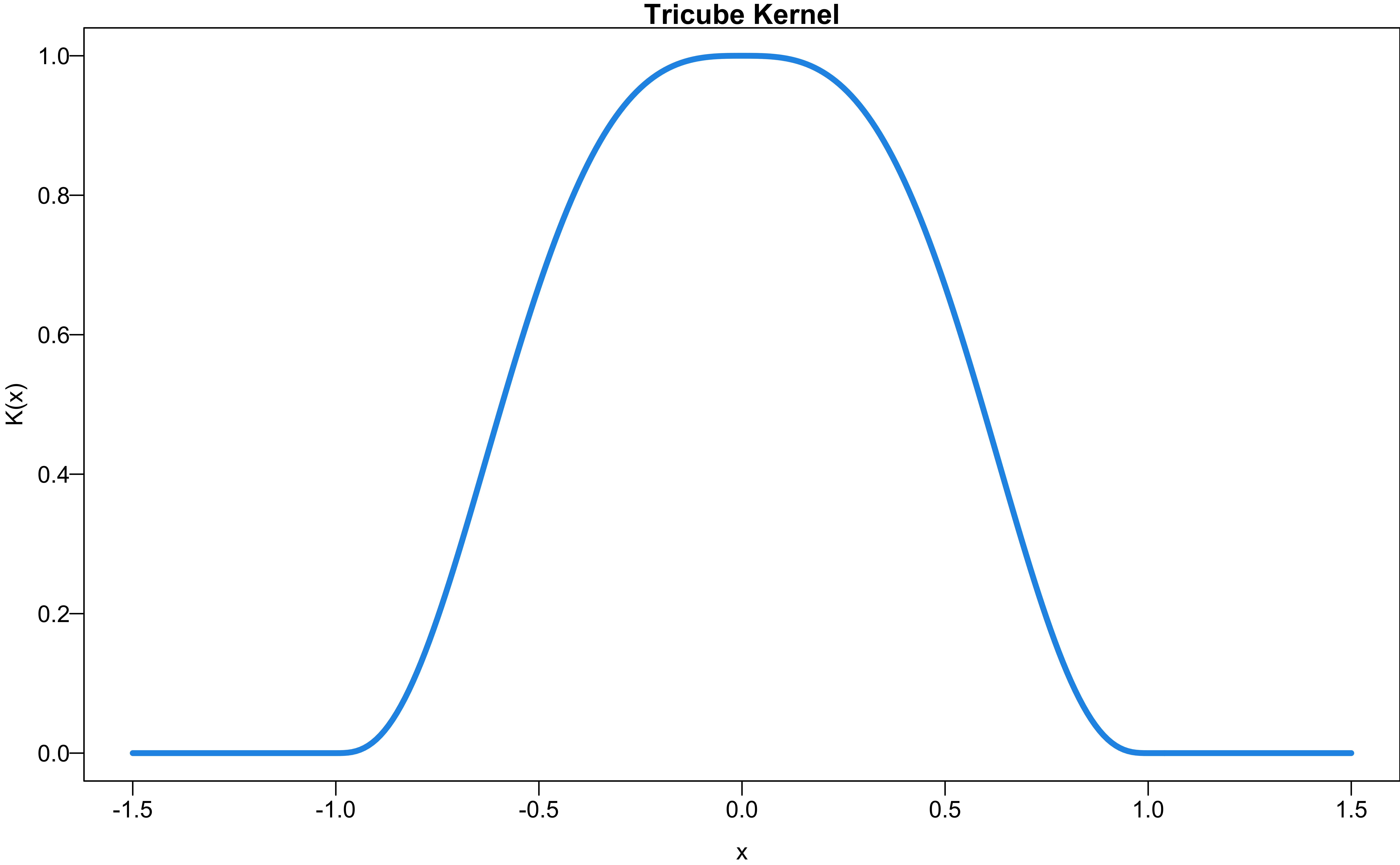
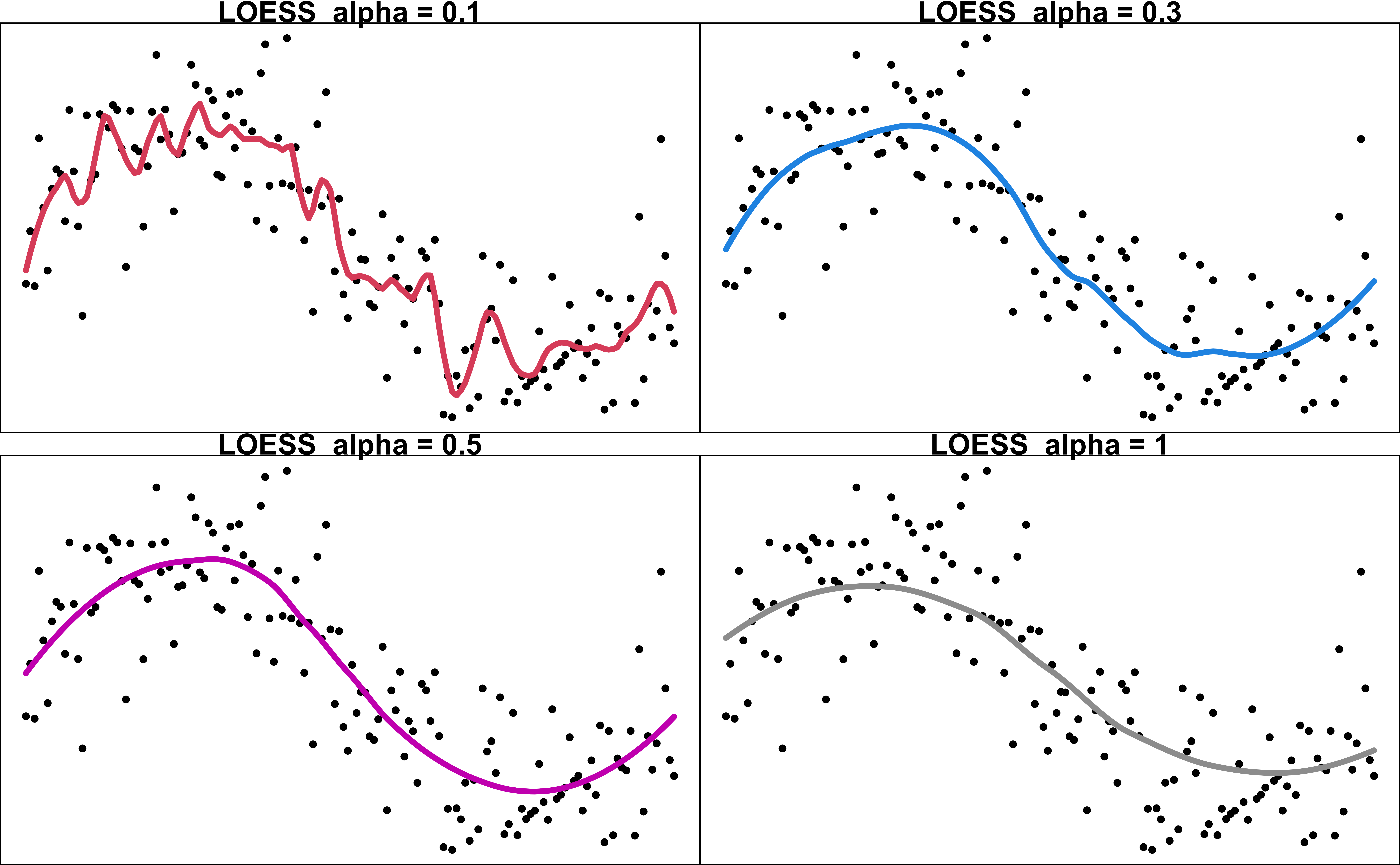
• The neighborhood \(N(x_0)\) is defined by the span parameter \(\alpha\), the fraction of the total points closest to \(x_0\).

loess(y ~ x, span = 0.75, degree = 2) ## Default setting

• Larger \(\alpha\) means more neighbors and smoother fitting.

LOESS is a special case of Local Polynomial Regression Fitting

LOESS Example

• LOESS uses the points in \(N(x_0)\) to generate a WLS estimate of \(y(x_0)\).

• LOESS is a special case of local polynomial regression.

R Implementation

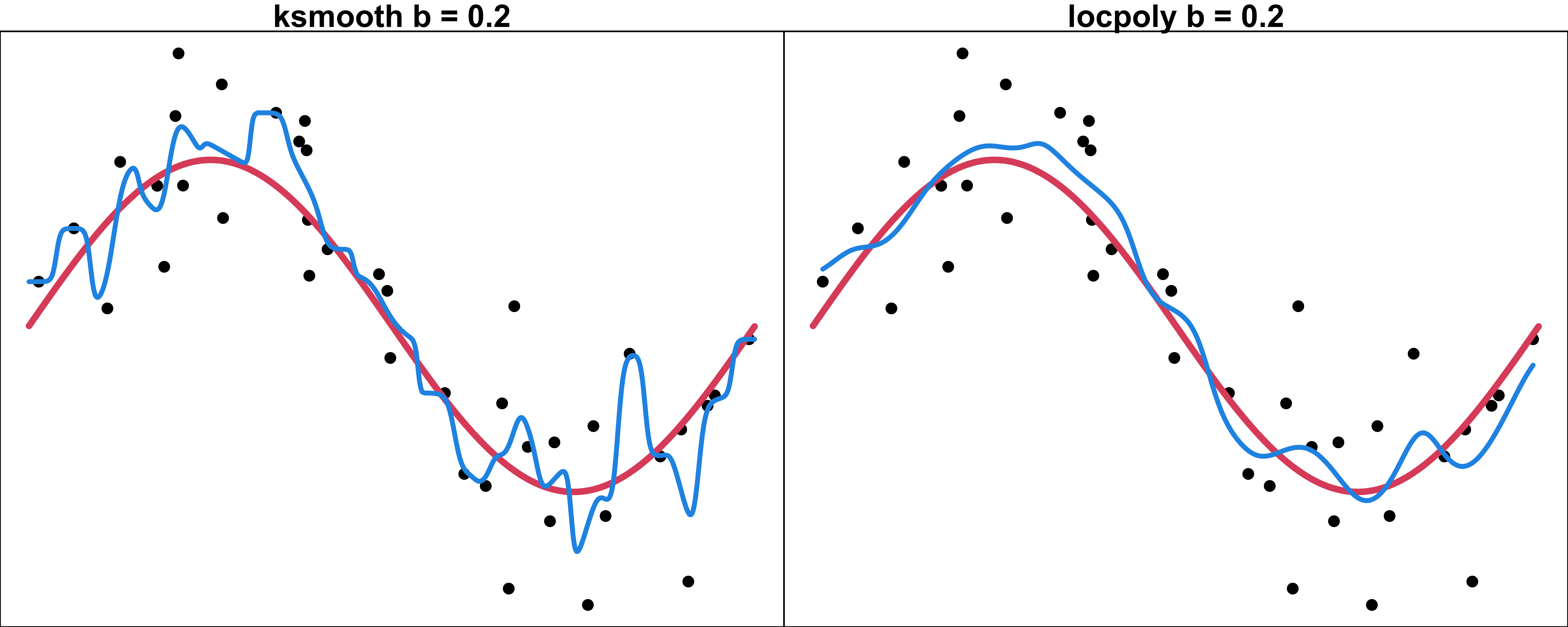
• loess(), KernSmooth::locploy(), locfit::locfit(), ksmooth(). Not all of them uses the same definition of the bandwidth.

• ksmooth: The kernels are scaled so that their quartiles are at \(\pm 0.25 * \text{bandwidth}\).

• KernSmooth::locpoly uses the raw value that we directly plug into the kernel.

• h=1.06σxn−1/5
• ksmooth: The kernels are scaled so that their quartiles (viewed as probability densities) are at ± 0.25*bandwidth.
• span: In this case, the bandwidth is decided by first finding the closes k neighbors and then use a tri-cubic weighting on the range of these neighbors. the bandwidth essentially varies depending on the target point
• the kknn() also utilize such a feature as default, so when you want to fit the standard KNN, you should specify method = “rectangular”, otherwise, the neighboring points will not receive the same weight.