Polynomial Regression ▶️

MATH 4780 / MSSC 5780 Regression Analysis

Dr. Cheng-Han Yu
Department of Mathematical and Statistical Sciences
Marquette University

Polynomial Regression

Polynomial Models in One Variable

Piecewise Regression

Splines

Why Polynomial Regression

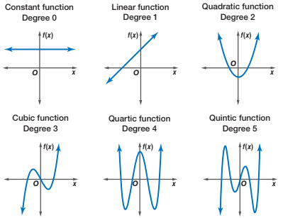
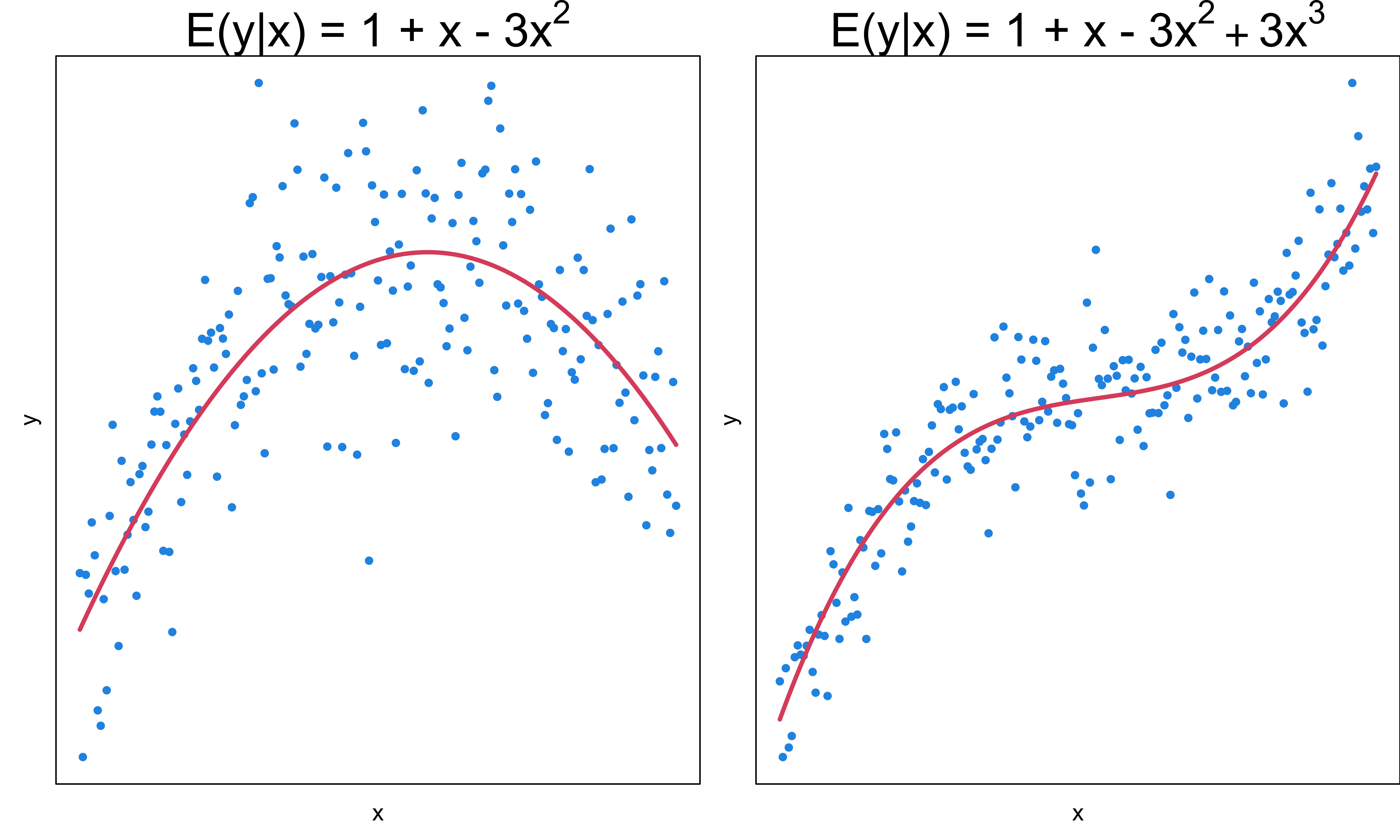
• Polynomials are widely used in situations where the response surface is curvilinear.
• Many complex nonlinear relationships can be adequately modeled by polynomials over reasonably small ranges of the \(x\)’s.

• They are also useful as approximating functions to unknown and possibly very complex nonlinear relationships.
• In this sense, the polynomial model is just the Taylor series expansion of the unknown function.

Polynomial Regression Models

• A second-order (degree) polynomial in one variable or a quadratic model is \[y = \beta_0 + \beta_1 x + \beta_2 x^2 + \epsilon\]

• A second-order polynomial in two variables is \[y = \beta_0 + \beta_1 x_1 + \beta_2 x_2 + \beta_{11}x_1^2 + \beta_{22}x_2^2 + \beta_{12}x_1x_2 + \epsilon\]

• The \(k\)th-order polynomial model in one variable is \[y = \beta_0 + \beta_1 x + \beta_2 x^2 + \cdots + \beta_kx^k + \epsilon\]

• If we set \(x_j = x^j\), this is just a multiple linear regression model with \(k\) predictors \(x_1, x_2, \dots, x_k\)!

Important Considerations

Keep the order of the model as low as possible.

• Transform data to keep the model 1st order.

• If fails, try a 2nd order model.

• Avoid higher-order polynomials unless they can be justified for reasons outside the data.

• 👉 Occam’s Razor: among competing models that predict equally well, choose the “simplest” one, i.e., a parsimonious model.

  • This avoids overfitting that leads to nearly perfect fit to the data, but bad prediction performance.

Source: Wikiversity

There are several important considerations that arise when fitting a polynomial in one variable. - A low-order model in a transformed variable is almost always preferable to a high-order model in the original metric. - Arbitrary fitting of high-order polynomials is a serious abuse of regression analysis. - You can always fit a polynomial model with very high order. It may give you a pretty good fit, but with very high chance, it will end up with very bad prediction, leading to overfitting. + Occam’s Razor: among competing models that predict equally well, choose the “simplest” one, i.e., parsimonious model. + This avoid overfitting that leads to bad prediction performance.

“Bayesian Deep Learning and a Probabilistic Perspective of Generalization” Wilson and Izmailov (2020) for the rationale of choosing a super high-order polynomial as the regression model.

• the ground truth explanation for the data is out of class for any of these choices, but there is some setting of the coefficients in choice (3) which provides a better description of reality than could be managed by choices (1) and (2).
• our beliefs about the generative processes for our observations, which are often very sophisticated, typically ought to be independent of how many data points we happen to observe.
• we often use neural networks with millions of parameters to fit datasets with thousands of points

Important Considerations

Model building strategy

• 👉 Forward selection: successively fit models of increasing order until the \(t\)-test for the highest order term is non-significant.

• 👉 Backward elimination: fit the highest order model and then delete terms one at a time until the highest order remaining term has a significant \(t\) statistic.

• 👉 They do not necessarily lead to the same model.

• 👉 Restrict our attention to low-order polynomials.

Important Considerations

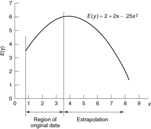
Extrapolation

• Can be extremely dangerous when the model is higher-order polynomial.
• The nature of the true underlying relationship may change or be completely different from the system that produced the data used to fit the model.

Important Considerations

Ill-conditioning

• Ill-conditioning: as the order of the model increases, \({\bf X'X}\) matrix inversion will become inaccurate, and error may be introduced into the parameter estimates
• Centering the predictors may remove some ill conditioning but not all.
• One solution is to use orthogonal polynomials (LRA Sec 7.5).

• Ill-conditioning refers to the fact that as the order of the model increases, \({\bf X'X}\) matrix inversion will become inaccurate, and error can be introduced into the parameter estimates
• Centering the predictors may remove some ill conditioning but not all.

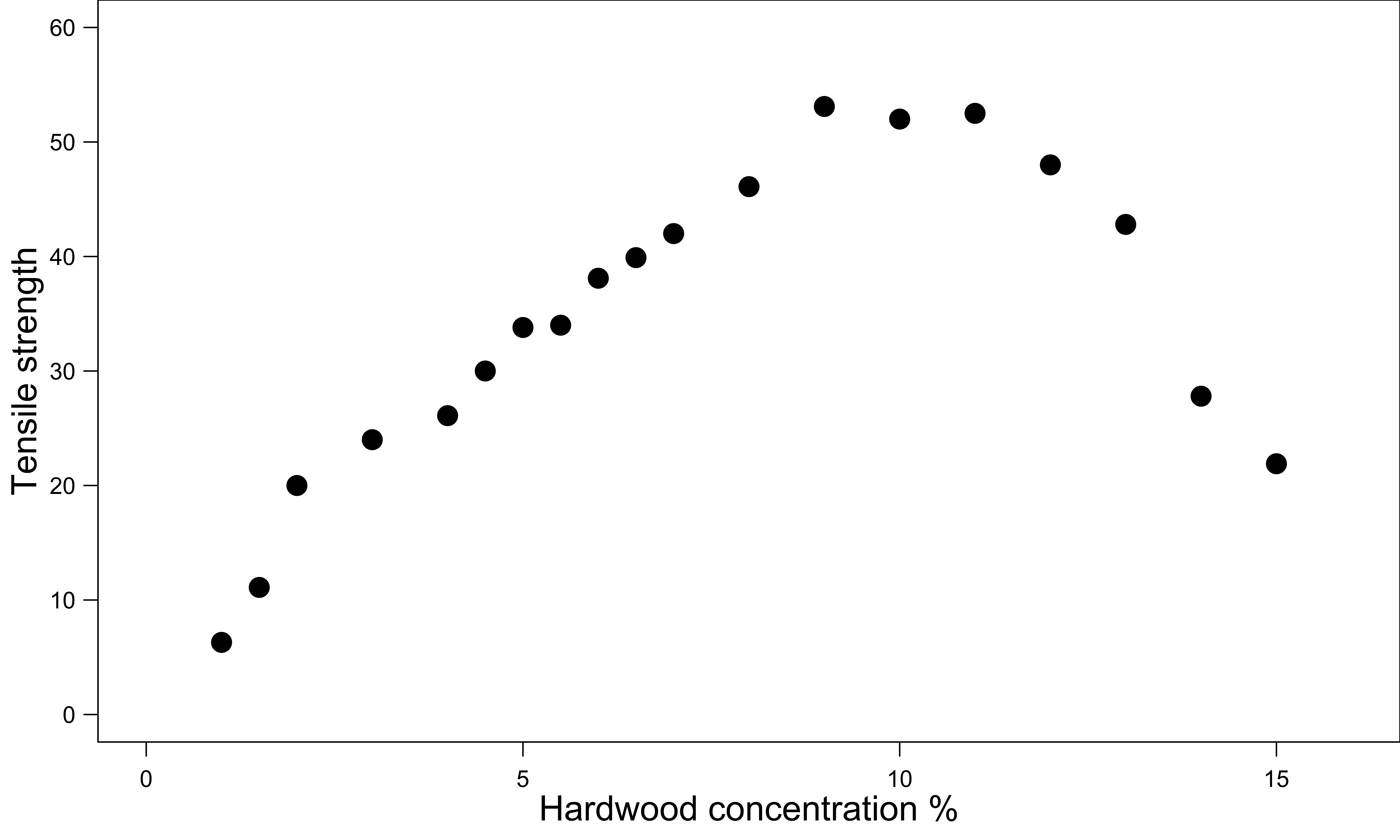
Example 7.1: Hardwood Data (LRA)

• Strength of kraft paper vs. the percentage of hardwood in the batch of pulp from which the paper was produced.
• A quadratic model may adequately describe the relationship between tensile strength and hardwood concentration.

hardwood[1:9, ]

  conc strength
1  1.0      6.3
2  1.5     11.1
3  2.0     20.0
4  3.0     24.0
5  4.0     26.1
6  4.5     30.0
7  5.0     33.8
8  5.5     34.0
9  6.0     38.1

R Lab Hardwood Data Model Fitting

• Following the suggestion that centering the data may remove nonessential ill-conditioning: \[y = \beta_0 + \beta_1 (x - \bar{x}) + \beta_2 (x - \bar{x}) ^ 2 + \epsilon\]

conc_cen <- hardwood$conc - mean(hardwood$conc)
lm(strength ~ conc_cen + I(conc_cen ^ 2), data = hardwood)

Call:
lm(formula = strength ~ conc_cen + I(conc_cen^2), data = hardwood)

Coefficients:
  (Intercept)       conc_cen  I(conc_cen^2)  
       45.295          2.546         -0.635  

• \(y = 45.3 + 2.55 (x - 7.26) - 0.63 (x - 7.26) ^ 2 + \epsilon\)
• Inference, prediction and residual diagnostics procedures are the same as multiple linear regression.

• We don’t need to create an extra predictor concentration ^ 2 in the data set.
• We can construct the x_sq term in the lm() function.
• We use I() function to wrap up the operation concen_cen ^ 2, so that concen_cen ^ 2 is not interpreted as a part of formula, but actual arithmetic operation.
• To avoid this confusion, the function I() can be used to bracket those portions of a model formula where the operators are used in their arithmetic sense. For example, in the formula y ~ a + I(b+c), the term b+c is to be interpreted as the sum of b and c.

Piecewise (Polynomial) Regression

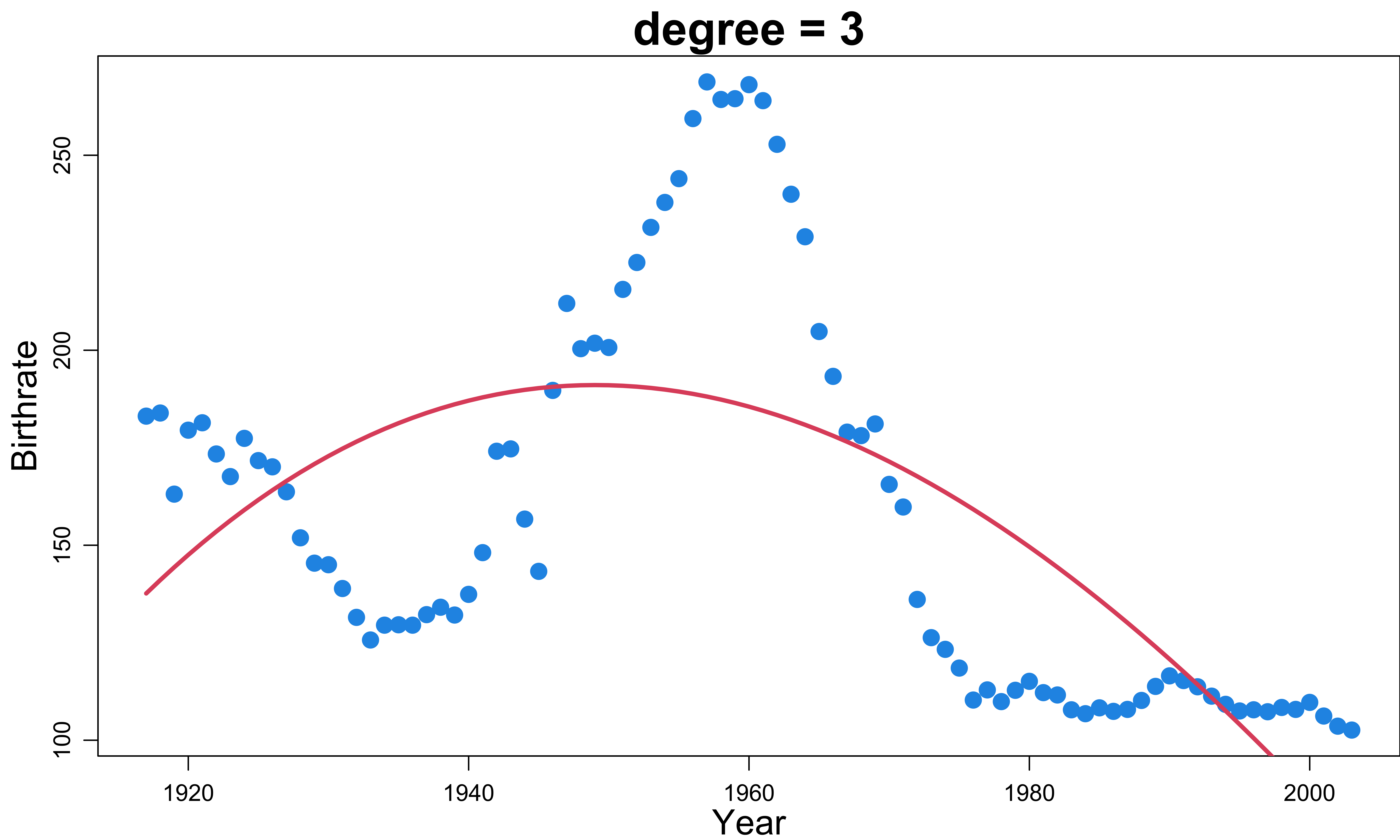
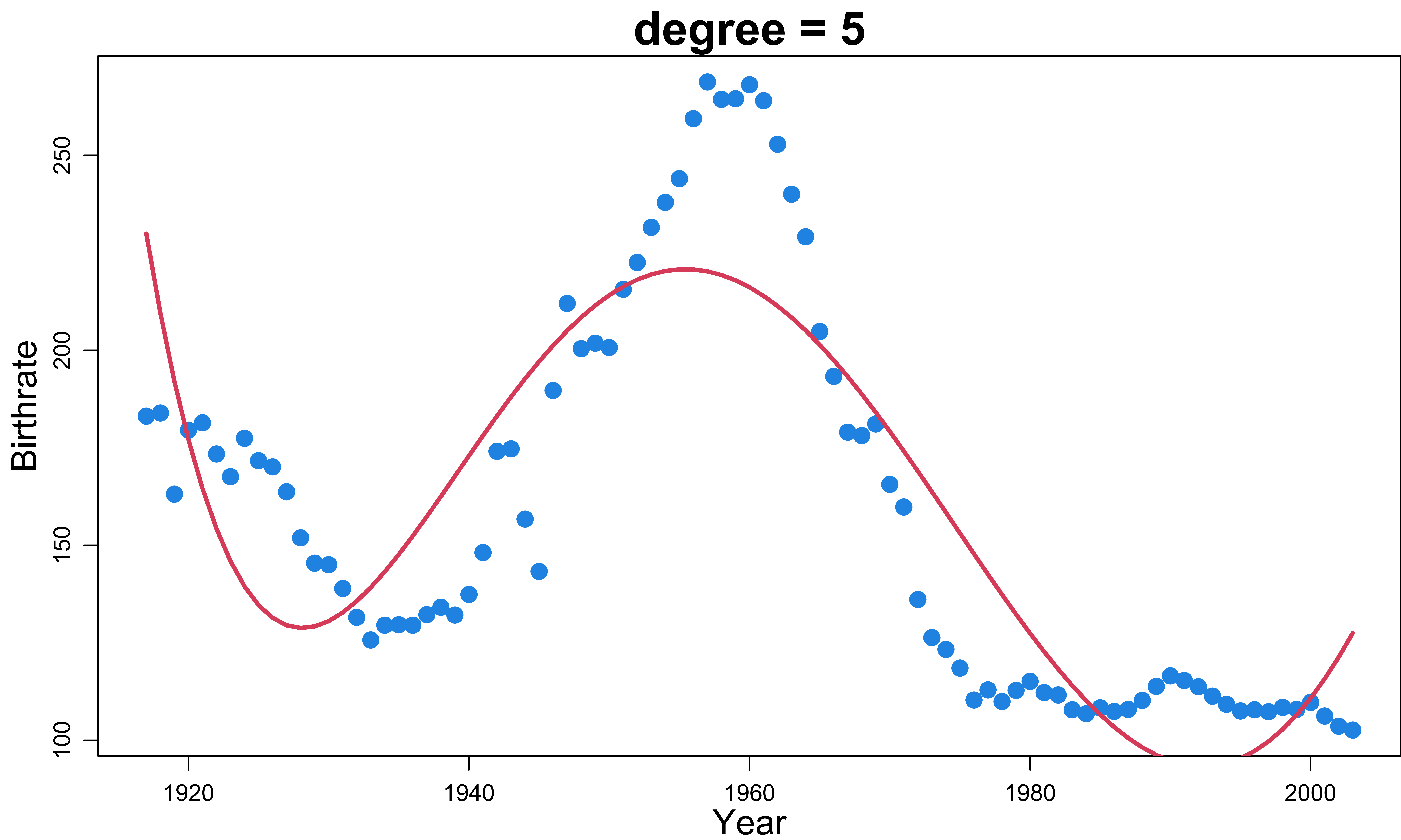
• A polynomial regression may provide a poor fit, and increasing the order does not improve the situation.
• This may happen when the regression function behaves differently in different parts of the range of \(x\).

• SOLUTION: 👉 piecewise polynomial regression that fits separate polynomials over different regions of \(x\).

• Example: \[y=\begin{cases} \beta_{01} + \beta_{11}x+ \beta_{21}x^2+\beta_{31}x^3 +\epsilon & \quad \text{if } x < c\\ \beta_{02} + \beta_{12}x+ \beta_{22}x^2+\beta_{32}x^3+\epsilon & \quad \text{if } x \ge c \end{cases}\]

• The joint points of pieces are called knots.

• Using more knots leads to a more flexible piecewise polynomial.

With \(K\) different knots, how many different polynomials do we have?

• There might be tow different systems or schemes that govern the relationship between response and predictor variables.
• Any issue of fitting a piecewise polynomial regression?
• In other words, we fit two different polynomial functions to the data, one on the subset of the observations with \(xi < c\), and one on the subset of the observations with \(xi ≥ c\). The first polynomial function has coefficients β01, β11, β21, β31, and the second has coefficients β02, β12, β22, β32.
• Each of these polynomial functions can be fit using least squares applied to simple functions of the original predictor.
• the function is discontinuous
• locations of the knots are known, otherwise it is a nonlinear regression problem.
• WE could fit piecewise regression with order 1.
• (or more constrained?)

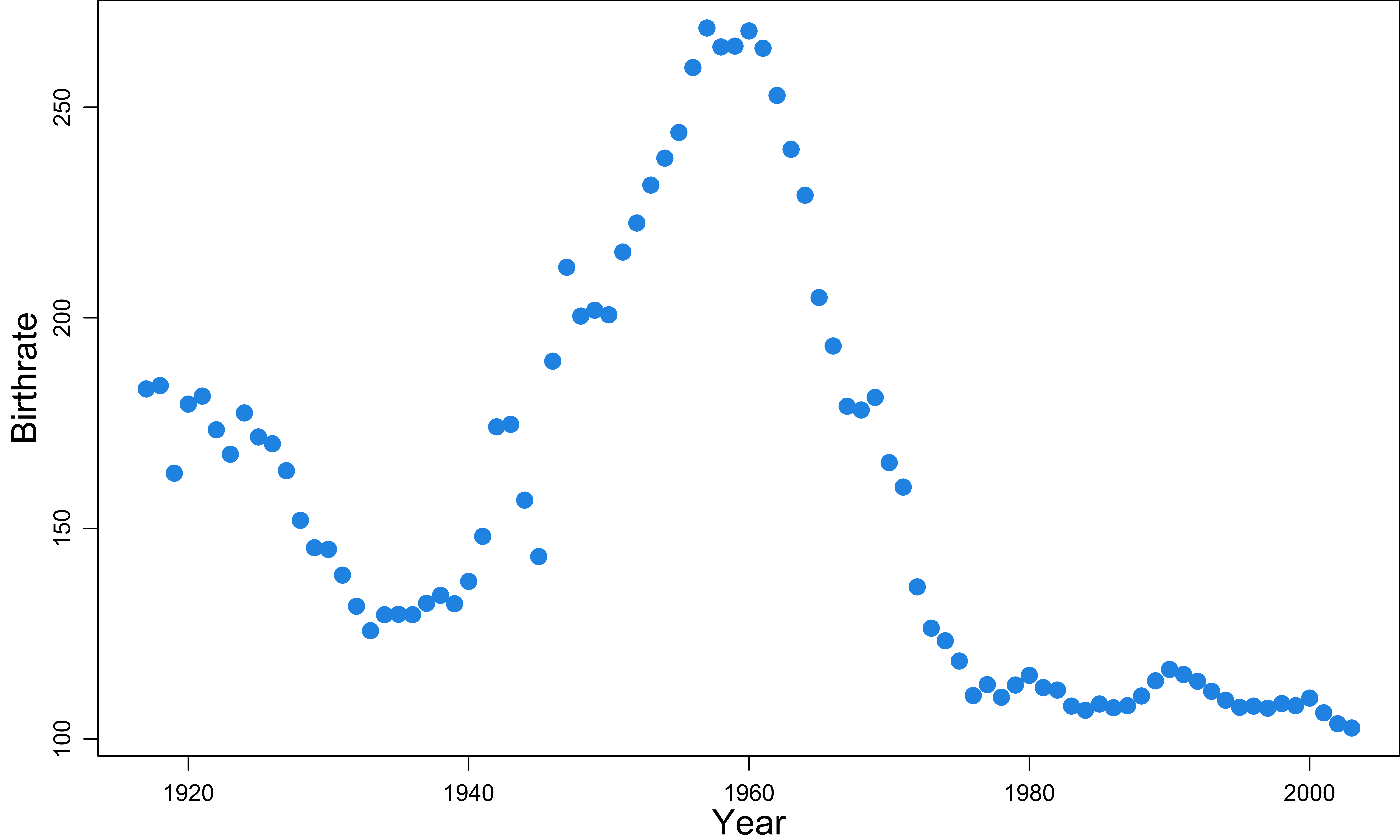
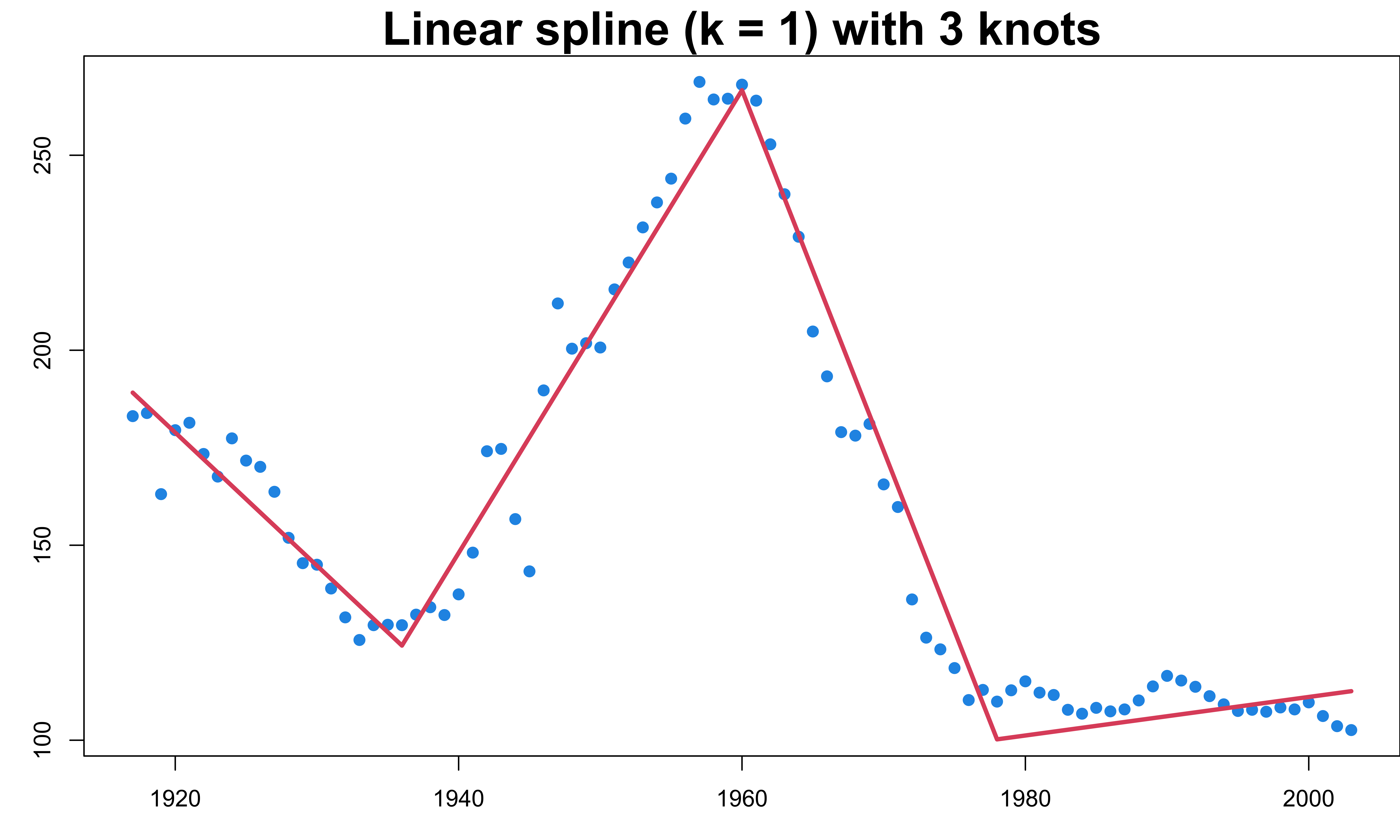
U.S. Birth Rate from 1917 to 2003

     Year Birthrate
1917 1917       183
1918 1918       184
1919 1919       163
1920 1920       180
1921 1921       181
1922 1922       173
1923 1923       168
1924 1924       177
1925 1925       172
1926 1926       170
1927 1927       164
1928 1928       152
1929 1929       145
1930 1930       145
1931 1931       139
1932 1932       132
1933 1933       126
1934 1934       130
1935 1935       130
1936 1936       130

R Lab A Polynomial Regression Provide a Poor Fit

lmfit3 <- lm(Birthrate ~ poly(Year - mean(Year), degree = 3, raw = TRUE),  
             data = birthrates)

It might be interesting to fit a linear regression with high order polynomials to approximate this curve. This can be carried out using the poly() function, which calculates all polynomials up to a certain power. Please note that this is a more stable method compared with writing out the powers such as I(Year^2), I(Year^3) etc because the Year variable is very large, and is numerically unstable.

R Lab Piecewise Polynomials: 3 knots at 1936, 60, 78

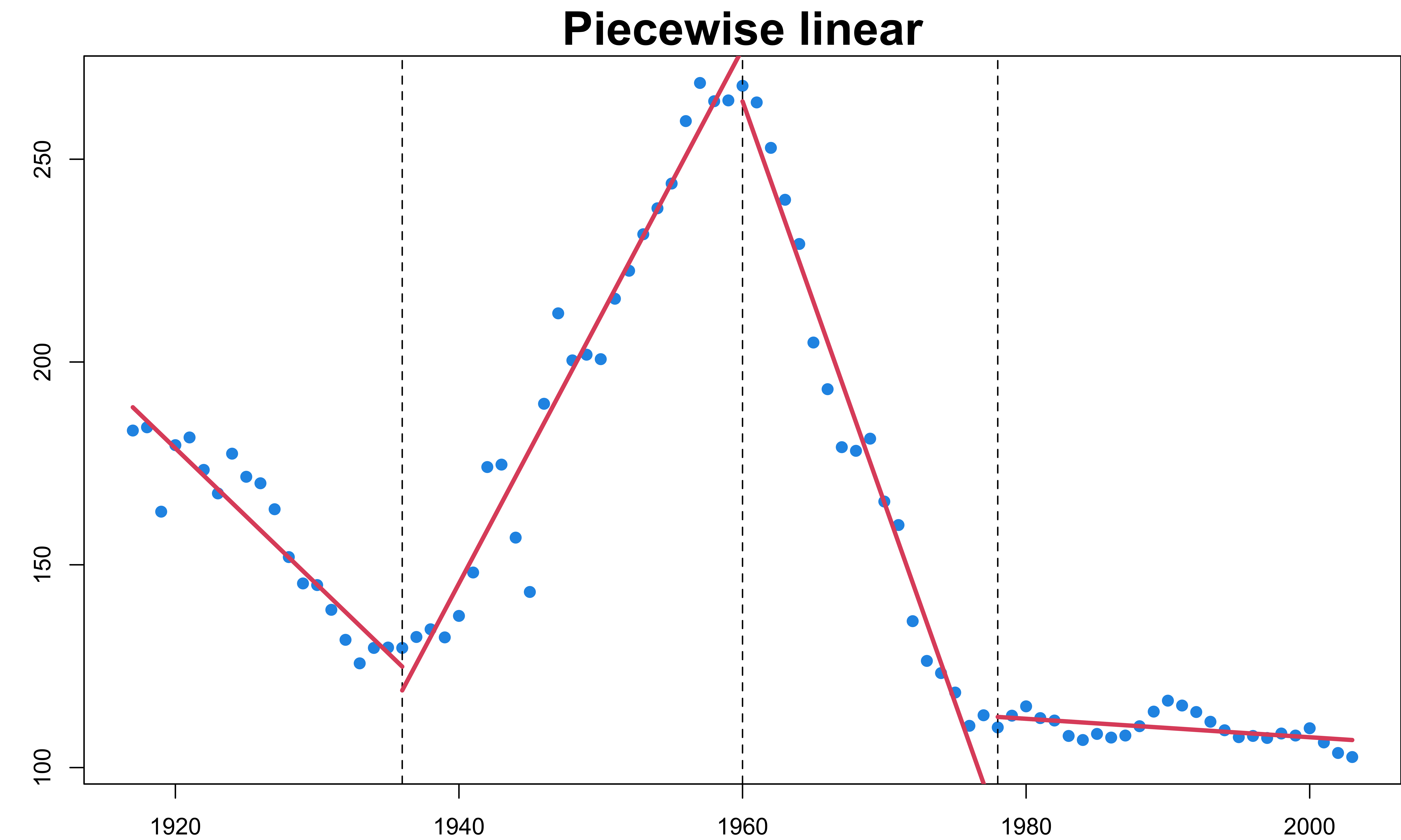
Any issue of piecewise polynomials?

these functions are not continuous. Hence we use a trick to construct continuous basis

Splines

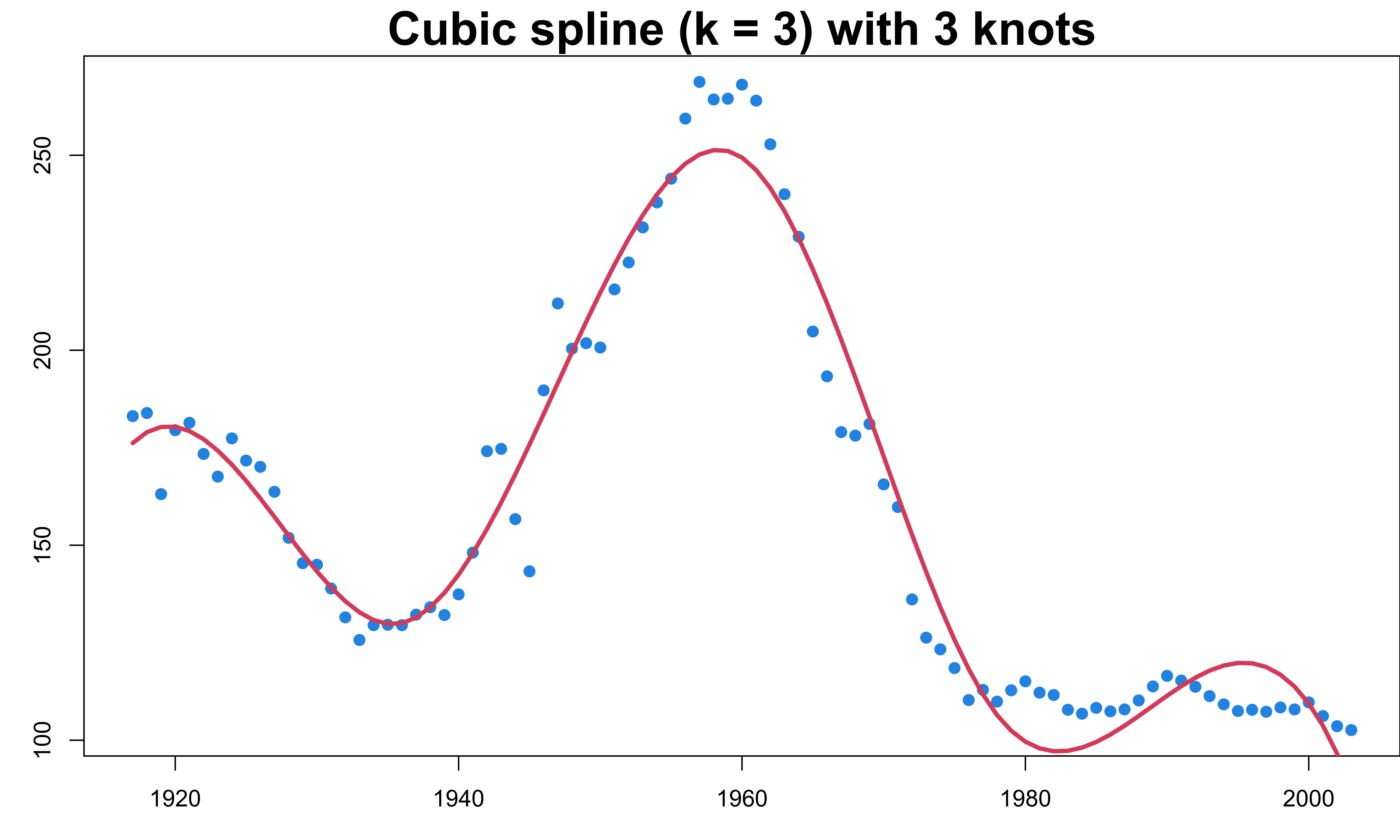
Splines of degree \(k\) are piecewise polynomials of degree \(k\) with continuity in derivatives (smoothing) up to degree \(k-1\) at each knot.

• Use bs() function in the splines package.

lin_sp <- lm(Birthrate ~ splines::bs(Year, degree = 1, knots = c(1936, 1960, 1978)), 
             data = birthrates)

Cubic Splines

• The cubic spline is a spline of degree 3 with first 2 derivatives are continuous at the knots.

cub_sp <- lm(Birthrate ~ splines::bs(Year, degree = 3, knots = c(1936, 1960, 1978)), 
             data = birthrates)

Practical Issue

• How many knots should be used
  • As few knots as possible
  • At least 5 data points per segment
• Where to place the knots
  • No more than one extreme point per segment
  • If possible, the extreme points should be centered in the segment
• What is the degree of functions in each region
  • Cubic spline is popular