Regression Diagnostics - Linearity ⏯

MATH 4780 / MSSC 5780 Regression Analysis

Dr. Cheng-Han Yu
Department of Mathematical and Statistical Sciences
Marquette University

Model Adequacy Checking and Correction

Non-normality

Non-constant Error Variance

Non-linearity and Lack of Fit

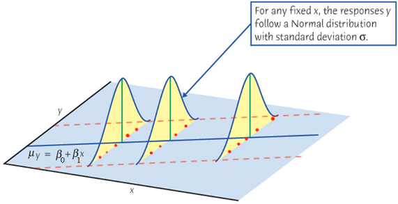
Assumptions of Linear Regression

\(Y_i= \beta_0 + \beta_1X_{i1} + \beta_2X_{i2} + \dots + \beta_kX_{ik} + \epsilon_i\)

• \(E(Y \mid X)\) and \(X\) are linearly related.
• \(\small E(\epsilon_i) = 0\)
• \(\small \mathrm{Var}(\epsilon_i) = \sigma^2\)
• \(\small \mathrm{Cov}(\epsilon_i, \epsilon_j) = 0\) for all \(i \ne j\).
• \(\small \epsilon_i \stackrel{iid}{\sim} N(0, \sigma^2)\) (for statistical inference)

• Assuming \(E(\epsilon) = 0\) implies that the regression surface captures the dependency of the conditional mean of \(y\) on the \(x\)s.
• Violating linearity implies that the model fails to represent the relationship between the mean response and the regressors. (Lack of fit)

Detecting Nonlinearity (CIA Example)

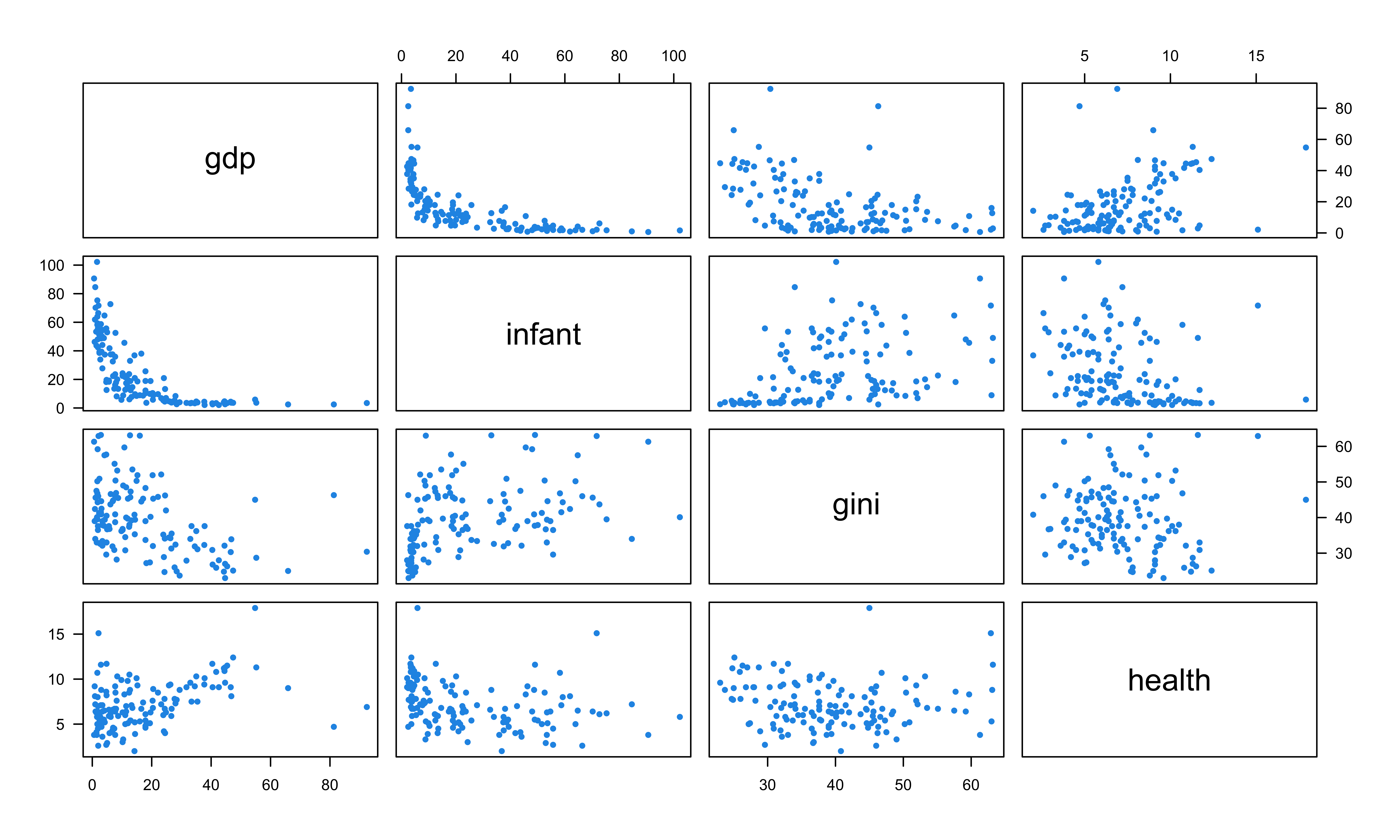
• Scatterplot \(y\) against each \(x\) can be misleading! It shows the marginal relationship between \(y\) and each \(x\), without controlling the level of other regressors.

Detecting Nonlinearity: Residual Plots

• Care about the partial relationship between \(y\) and each \(x\) with impact of other \(x\)s controlled.

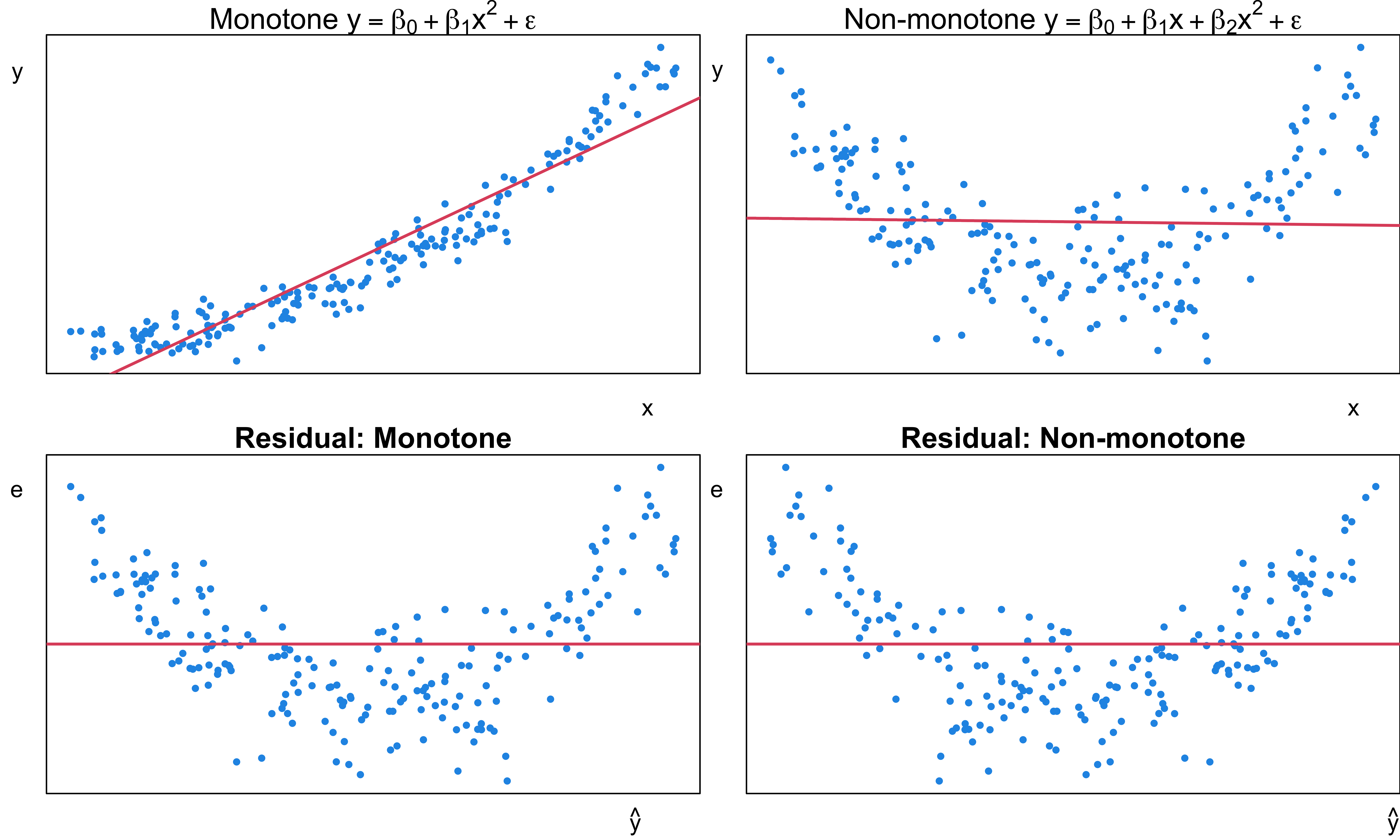
• Residual-based plots are more relevant in detecting the departure of linearity.

• Residual plots cannot distinguish between monotone and non-monotone nonlinearity.
• The distinction:
  • Monotone: just transform \(x\) to \(x^2\)
  • Non-monotone: need quadratic form

• The OLS ensures that the residuals and fitted values are uncorrelated.

Detecting Nonlinearity: Partial Residual Plots

• Partial residual plots (Component-plus-Residual Plot) are for diagnosing nonlinearity.

• The partial residuals for \(x_j\): \[e_i^{(j)} = b_jx_{ij} + e_i\]

  • \(b_j\) is the coefficient of \(x_j\) in the full multiple regression
  • \(e_i\)s are the residuals from the full multiple regression

• Partial residual plot \(e_i^{(j)}\) vs. \(x_{ij}\) for \(x_j\)

• The nonlinear pattern can be highlighted or emphasized
• Added-variable plots, for detecting influential data, are partial plots, but they don’t work well for detecting nonlinearity because they are biased towards linearity
• Cook (1993): if the regressions of x_j on the other xs are approximately linear, then the regression function in the crPlot provides a visualization of transformation.
• If the regressions among the predictors are strongly nonlinear and not well described by polynomials, then cvPlot may not be effective in recovering nonlinear partial relationships. => Use CERES plots (ceresPlots())
• And cvPlots can appear nonlinear even when the true partial regression is linear => called leakage.

R Lab Partial Residual Plots

logciafit <- lm(log(infant) ~ gdp + health + gini, data = CIA)
# Component-plus-Residual Plot 
car::crPlots(logciafit, ylab = "partial residual", layout = c(1, 3), grid = FALSE, main = "") 

Transformation for Linearity

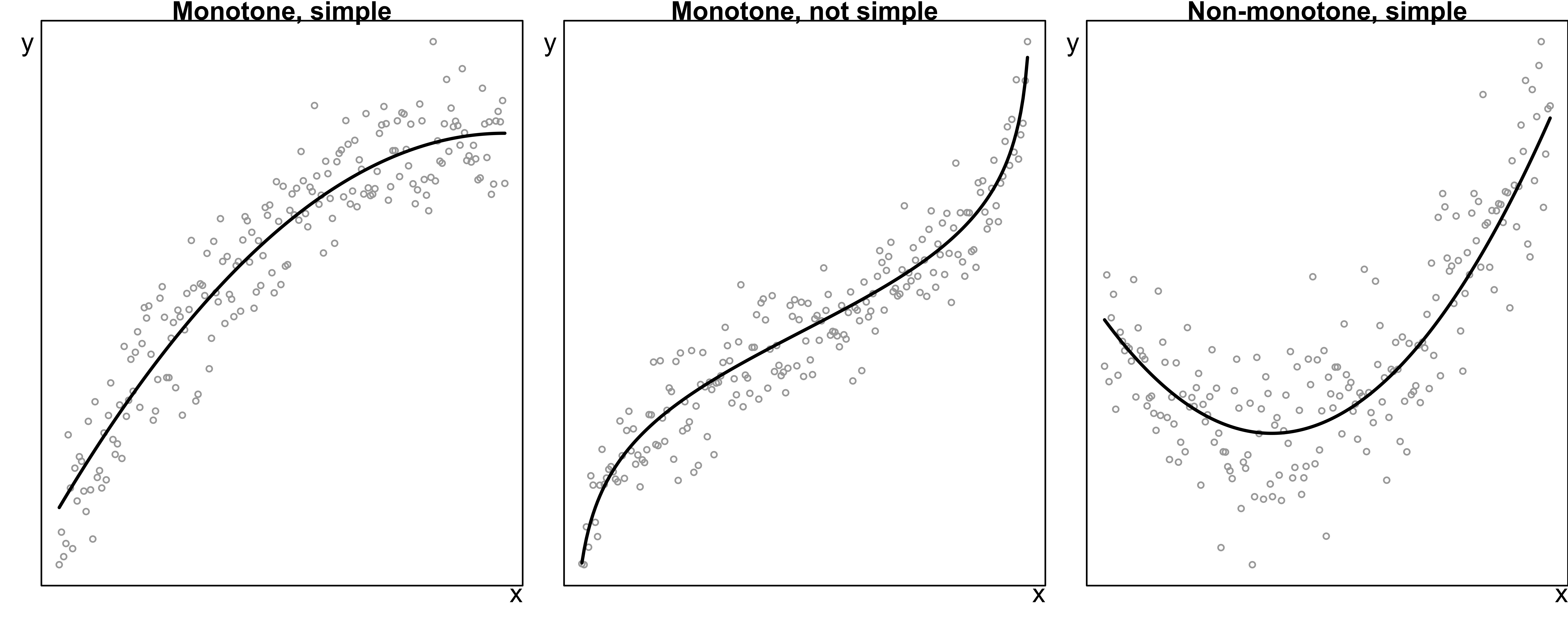
• Monotone, simple: Power transformation on \(x\) and/or \(y\)
• Monotone, not simple: Polynomial regression (next week) or regression splines (MSSC 6250)
• Non-Monotone, simple: Quadratic regression \(y = \beta_0 + \beta_1 x + \beta_2 x^2 + \epsilon\)

• not simple: direction of curvature changes
• Transform an \(x\) rather than \(y\), unless we see a common pattern of nonlinearity in the partial relationships of \(y\) to many \(x\)s.
• Transforming \(y\) changes the shape of its relationship to all of the \(x\)s, and also changes the shape of the residual distribution.

Bulging Rule for Simple Monotone Nonlinearity

The bulge points	Transform	Ladder of powers/roots
left	\(x\)	down, e.g., \(\log(x)\)
right	\(x\)	up
down	\(y\)	down
up	\(y\)	up

• Prefer to transform an \(x\) rather than \(y\), unless we see a common pattern of nonlinearity in the partial relationships of \(y\) to many \(x\)s.

Mosteller and Tukey’s (1977) - Transform an \(x\) rather than \(y\), unless we see a common pattern of nonlinearity in the partial relationships of \(y\) to many \(x\)s. - Transforming \(y\) changes the shape of its relationship to all of the \(x\)s, and also changes the shape of the residual distribution.

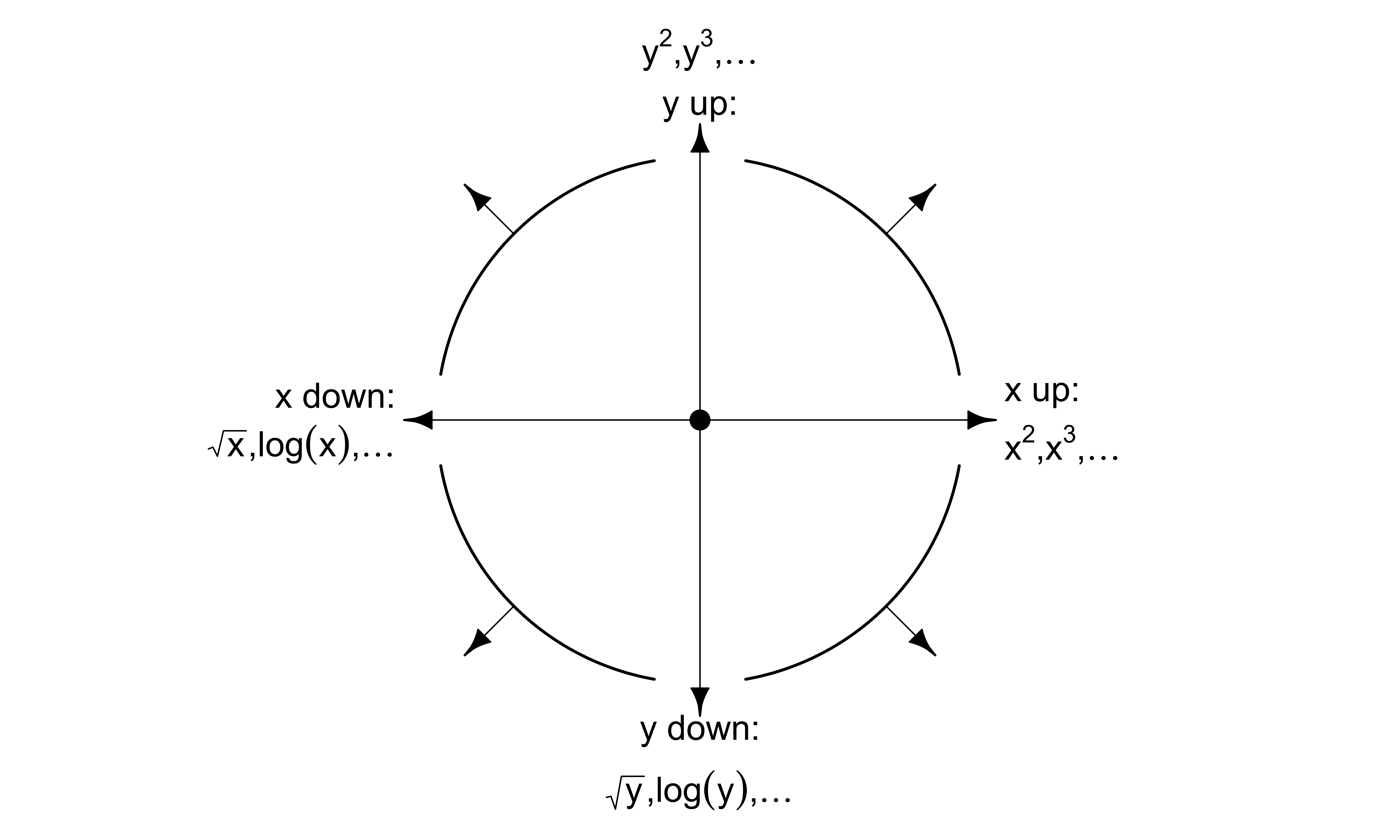
Transformation on \(x\)s

• gdp to log(gdp)
• health to health + health^2

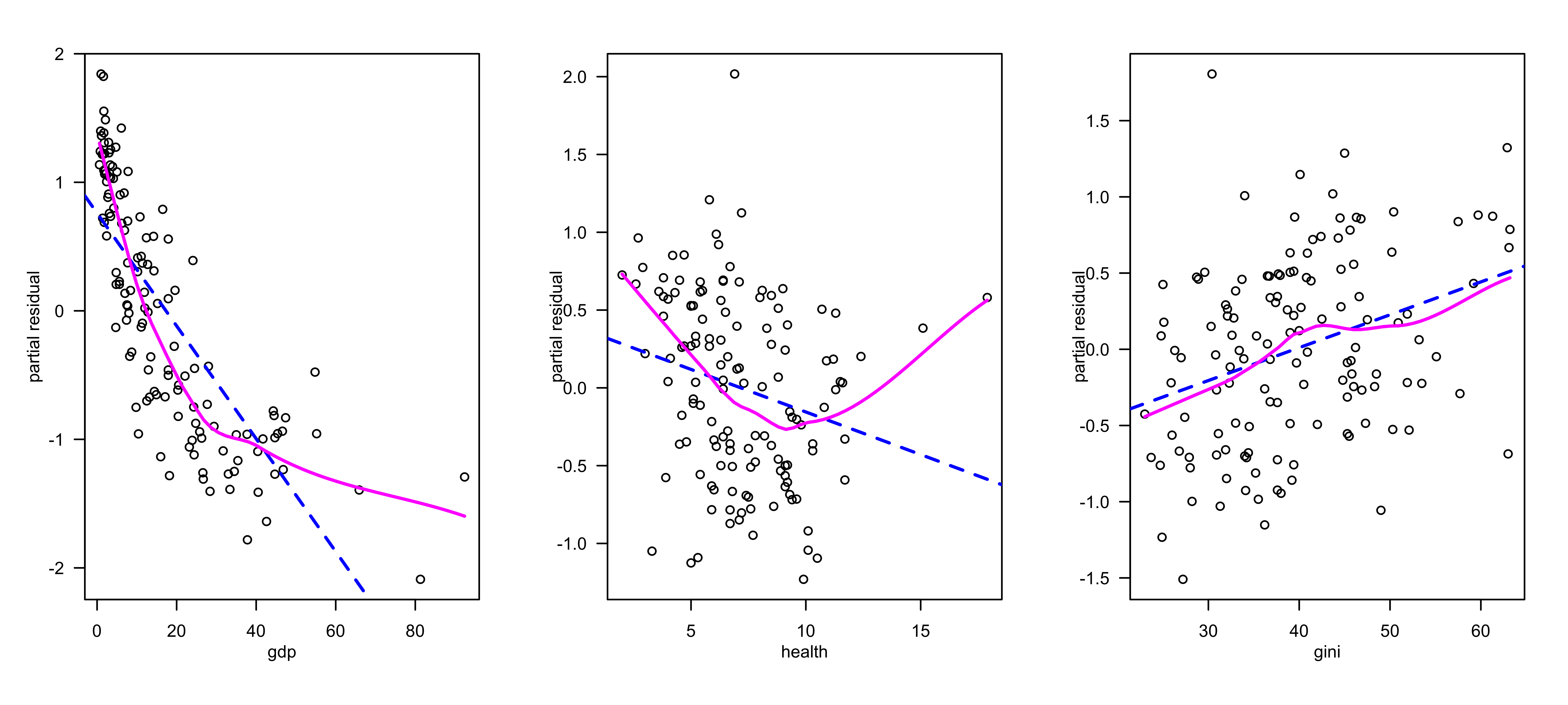
R Lab Partial Residual Plots

logciafit2 <- update(logciafit, . ~ log(gdp) + poly(health, degree = 2, raw = TRUE) + gini)
car::crPlots(logciafit2, ylab = "partial residual", layout = c(1, 3), grid = FALSE, main = "") 

if true, use raw and not orthogonal polynomials. - If the partial relationship of log(infant) to health expenditure is quadratic, its partial residual plot should be linear.

R Lab Improving Model Performance

car::brief(logciafit, digits = 2)

           (Intercept)     gdp health   gini
Estimate          3.02 -0.0439 -0.055 0.0216
Std. Error        0.29  0.0037  0.022 0.0061

 Residual SD = 0.59 on 130 df, R-squared = 0.71 

car::brief(logciafit2, digits = 2)

           (Intercept) log(gdp) poly(health, degree = 2, raw = TRUE)1
Estimate          4.65   -0.720                                -0.221
Std. Error        0.32    0.038                                 0.058
           poly(health, degree = 2, raw = TRUE)2   gini
Estimate                                  0.0096 0.0191
Std. Error                                0.0034 0.0044

 Residual SD = 0.44 on 129 df, R-squared = 0.84 

R Lab Plotting against Original Untransformed \(x\)

Code

library(effects)
par(mar = c(2, 2, 0, 0))
plot(Effect("gdp", logciafit2, residuals = TRUE), 
     lines = list(col = c("blue", "black"), lty = 2), 
     axes = list(grid = TRUE), confint = FALSE, 
     partial.residuals = list(plot = TRUE, smooth.col = "magenta", 
                              lty = 1, 
                              span = 3/4), 
     xlab = "GDP per Capita", ylab = "Partial Residual", main = "", cex.lab = 2)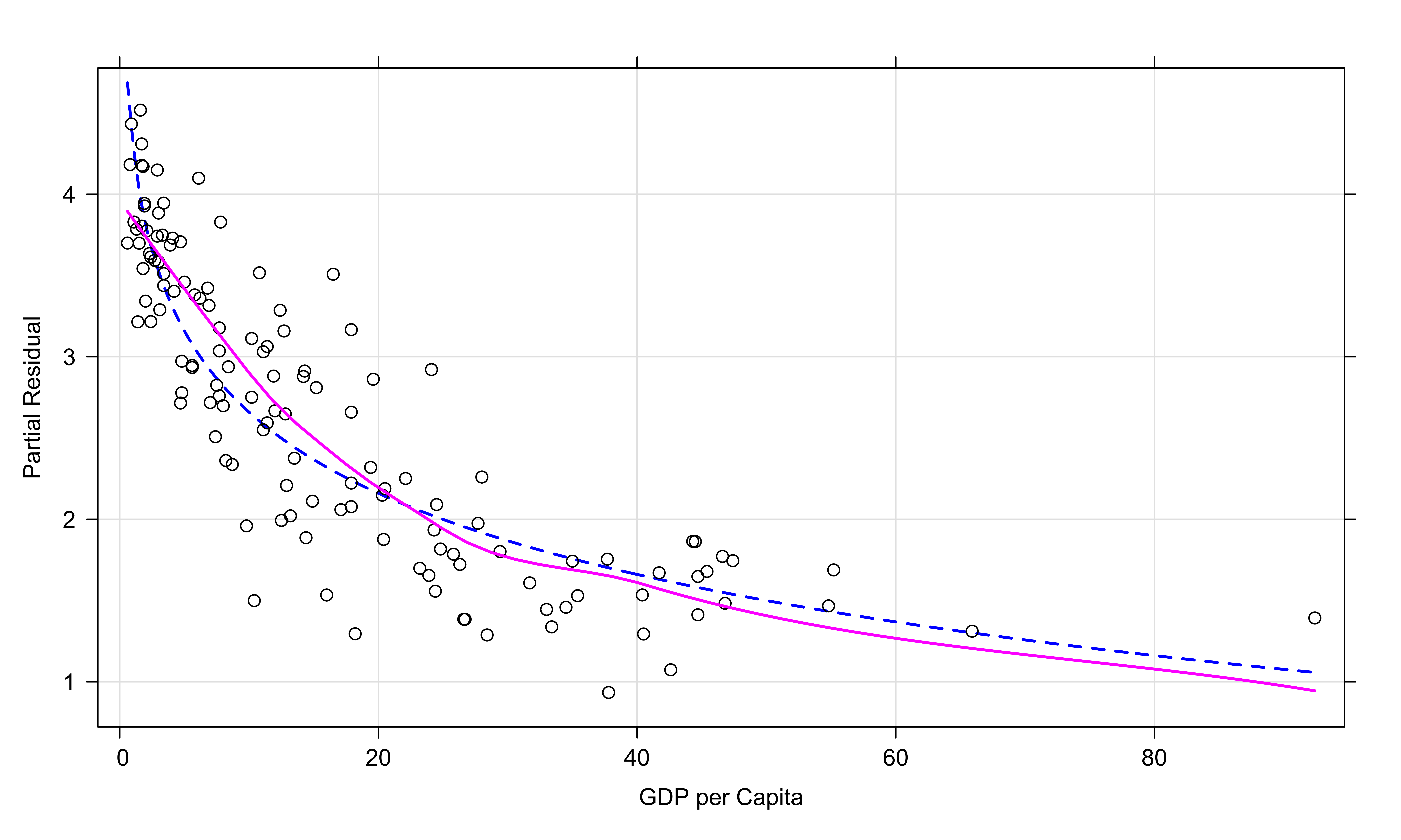

Code

par(mar = c(2, 2, 0, 0))
plot(Effect("health", logciafit2, residuals = TRUE), 
     lines = list(col = c("blue", "black"), lty = 2), 
     axes = list(grid = TRUE), confint = FALSE, 
     partial.residuals = list(plot = TRUE, smooth.col = "magenta", 
                              lty = 1, 
                              span = 3/4),
     xlab = "Health Expenditures", ylab = "Partial Residual", main = "", cex.lab = 2)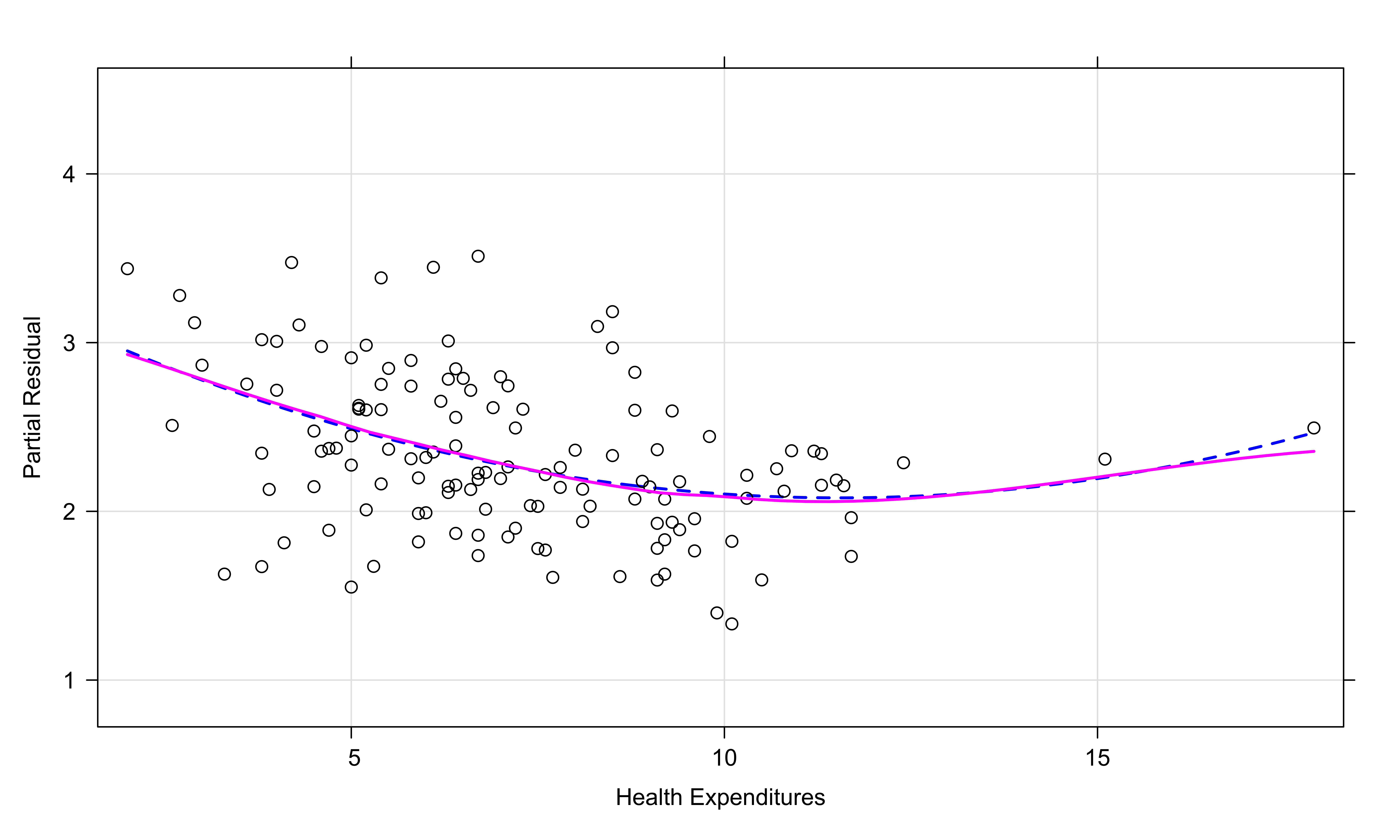

• plot(Effect(“gdp”, logciafit2, residuals = TRUE))

• \(\epsilon^{(1)}_i = f_1(x_{i1}) + e_i\) either if the partial-regression function \(f_1(x_1)\) is linear after all or if the other \(x\)s are each linearly related to \(x_1\).

• In practice, it’s only strongly nonlinearly related \(x\)s that seriously threaten the validity of component-plus-residuals plots.

• Correlation between x1 and x2 can induce spurious nonlinearity in the CR plot for x1.

• trying to correct nonlinearity for one x at a time, but in my experience, it’s rarely necessary to proceed sequentially.

Transforming \(x\)s Analytically: Box and Tidwell (1962)

• Box and Tidwell (1962) proposed a procedure for estimating \(\lambda_1, \lambda_2, \dots, \lambda_k\) in the model \[y = \beta_0 + \beta_1x_1^{\lambda_1} + \cdots + \beta_kx_k^{\lambda_k}+ \epsilon\]

• All \(x_j\)s are positive.

• \(\beta_0, \beta_1, \dots, \beta_k\) are estimated after and conditional on the transformations.

• \(x_j^{\lambda_j} = \log_e(x_j)\) if \(\lambda_j = 0\).

• If some of the xs (for instance, dummy regressors) aren’t candidates for transformation, then these xs can simply enter the model linearly.
• all positive xs

R Lab Box and Tidwell (1962)

Consider the model \[\log(Infant) = \beta_0 + \beta_1 GDP^{\lambda_1} + \beta_2Gini^{\lambda_2} + \beta_3 Health + \beta_4 Health ^ 2 + \epsilon\]

car::boxTidwell(log(infant) ~ gdp + gini, 
                other.x = ~poly(health, 2, raw = TRUE), data = CIA)

...
     MLE of lambda Score Statistic (t) Pr(>|t|)    
gdp            0.2                10.6   <2e-16 ***
gini          -0.5                -0.4      0.7    
---
Signif. codes:  0 '***' 0.001 '**' 0.01 '*' 0.05 '.' 0.1 ' ' 1
...

• The point estimate of \(\lambda\) is \(\hat{\lambda}_1 = 0.2\) and \(\hat{\lambda}_2 = -0.5\)

• The test is for \(H_0:\) No transformation is needed \((\lambda = 1)\).

  • Strong evidence to transform \(GDP\)
  • Little evidence of the need to transform the Gini coefficient

Other Methods for Dealing with Nonlinearity

• Lack-of-fit test (LRA Sec 4.5, CMR Sec. 3.6): Need repeated observations

• Transform a nonlinear function into a linear one (LRA Sec 5.3)

Can the nonlinear model \(y = \beta_0e^{\beta_1x}\epsilon\) be transformed into a linear one (intrinsically linear)?

• Polynomial Regression, Regression Splines or other nonparametric regression (MSSC 6250)

• A (pure) nonlinear model may be needed if the model assumptions cannot be satisfied.