Regression Diagnostics - Constant Variance 📖

MATH 4780 / MSSC 5780 Regression Analysis

Dr. Cheng-Han Yu
Department of Mathematical and Statistical Sciences
Marquette University

Model Adequacy Checking and Correction

Non-normality

Non-constant Error Variance

Non-linearity and Lack of Fit

• This week we are going to learn some methods to correct model inadequacy.
• We can either transform our data, our use a more general method, called Generalized Least Squares or Weighted Least Squares.
• \(\epsilon_i \stackrel{iid}{\sim} N(0, \sigma^2)\): mean 0, constant variance, normally distributed, and uncorrelated.
• \(E(\epsilon_i) =0\) implies the function form of the model (linearity) is correct.

Nonconstant Error Variance

Without constant variance,

• LSEs are still unbiased if linearity and independence of \(x\)s and errors hold.

• Inference results are not convincing: distorted \(p\)-values and incorrect coverage of confidence interval.

• The \(b_j\)s will have larger standard errors (no minimum-variance).

Is it harder or easier to reject \(H_0: \beta_j = 0\) when the standard error of \(b_j\) is larger?

• For these consequences to occur, nonconstant error variance must be severe.

Detecting Nonconstant Error Variance

• Common pattern: the conditional variation of \(y\) to increase with the level of \(y\).

• It seems natural to plot \(e_i\) against \(y\)

  • \(e_i\) have unequal variances \((\mathrm{Var}(e_i) = \sigma^2(1-h_{ii}))\) even when the errors \(\epsilon_i\) have equal variances \(\mathrm{Var}(\epsilon_i) = \sigma^2\).
  • \(e_i = y_i - \hat{y}_i\) are correlated with \(y\)

• Use R-student residual plot \(t_i\) vs. \(\hat{y}_i\) because R-student residuals have constant variance and they are uncorrelated with \(\hat{y}_i\).

\(r_{ey} = \sqrt{1-R^2}\) https://stats.stackexchange.com/questions/5235/what-is-the-expected-correlation-between-residual-and-the-dependent-variable

Residual Plots

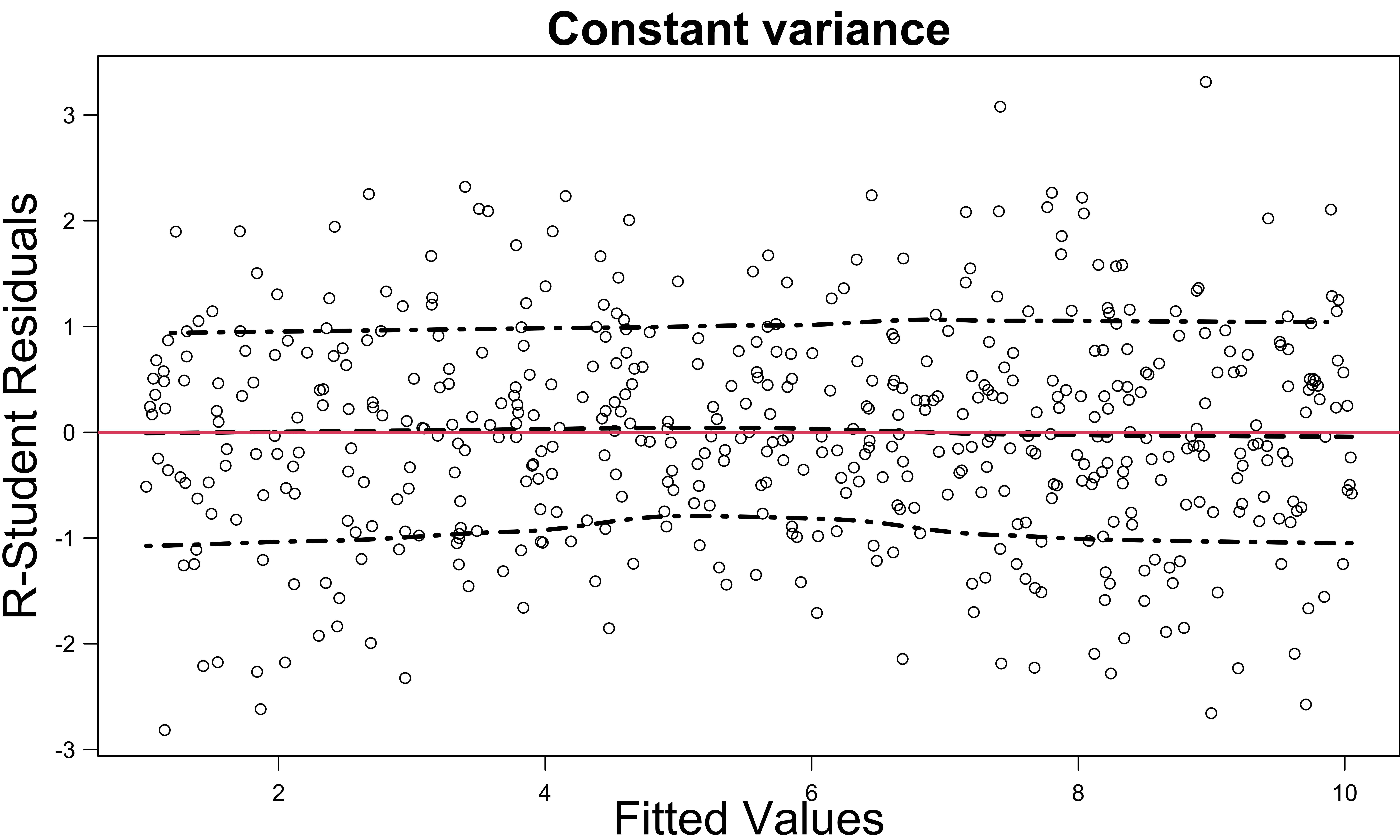
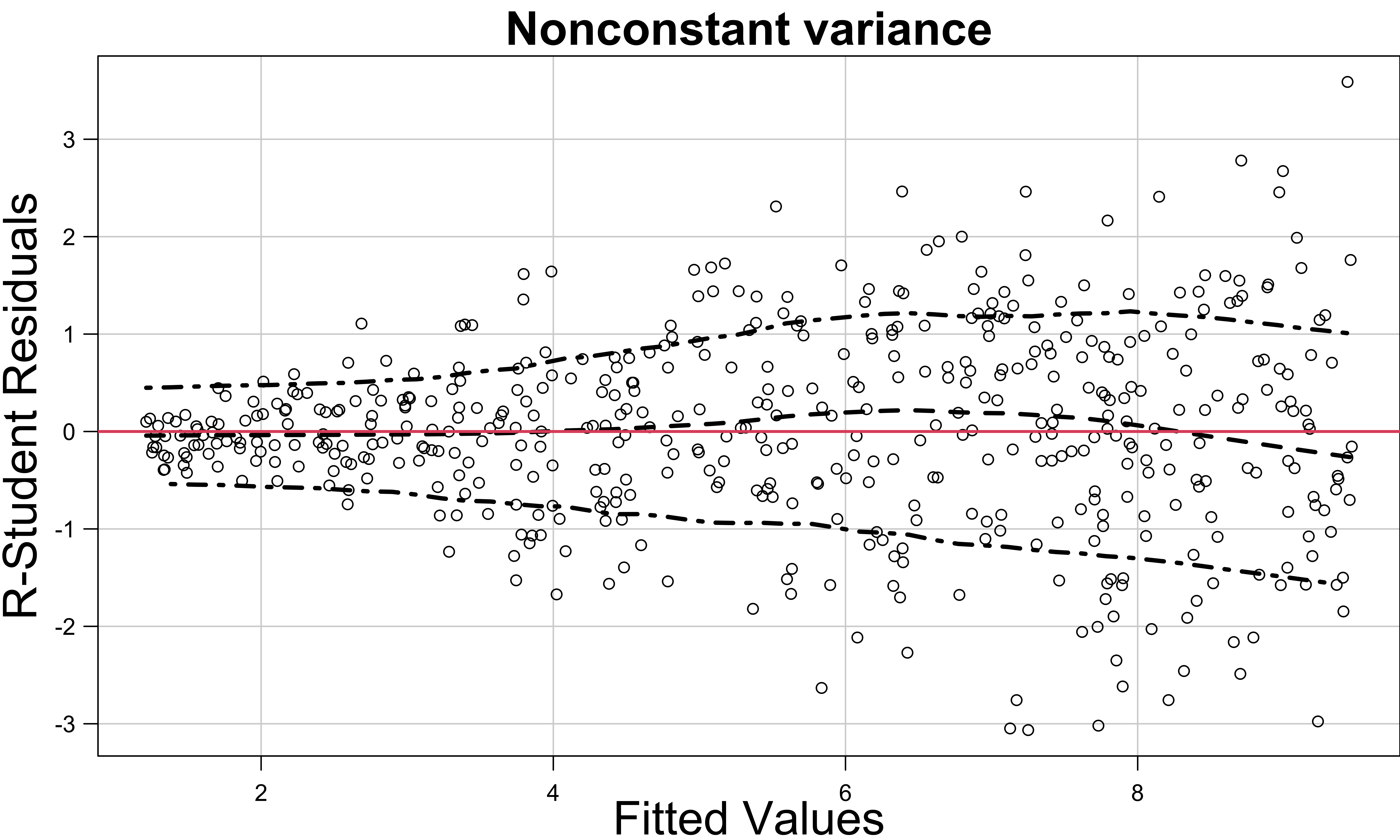
• If the spread of the residuals increases with the level of the fitted values, we might be able to correct the problem by transforming \(y\) down the ladder of power and roots.

Variance Stablizing Transformation

• Constant variance assumption is often violated when the response \(y\) follows a distribution whose variance is functionally related to mean.

Can you provide a distribution whose variance is functionally related to its mean?

Relationship of \(\sigma^2\) to \(E(y)\)	Transformation
\(\sigma^2 \propto\) constant	\(y' = y\) (no transformation)
\(\sigma^2 \propto E(y)\)	\(y' = \sqrt{y}\) (square root; Poisson)
\(\sigma^2 \propto E(y)[1-E(y)]\)	\(y' = \sin^{-1}(\sqrt{y})\) (arcsin; binomial proportions \(0 \le y_i \le 1\))
\(\sigma^2 \propto [E(y)]^2\)	\(y' = \ln(y)\) (natural log)
\(\sigma^2 \propto [E(y)]^3\)	\(y' = y^{-1/2}\) (reciprocal square root)
\(\sigma^2 \propto [E(y)]^4\)	\(y' = y^{-1}\) (reciprocal)

• The strength of a transformation depends on the amount of curvature that it induces
• a mild transformation applied over a relatively narrow range of values (e.g., y max / y min < 2, 3) has little effect. On the other hand, a strong transformation over a wide range of values will have a dramatic effect on the analysis.

R Lab Nonconstant Variance (CIA Example)

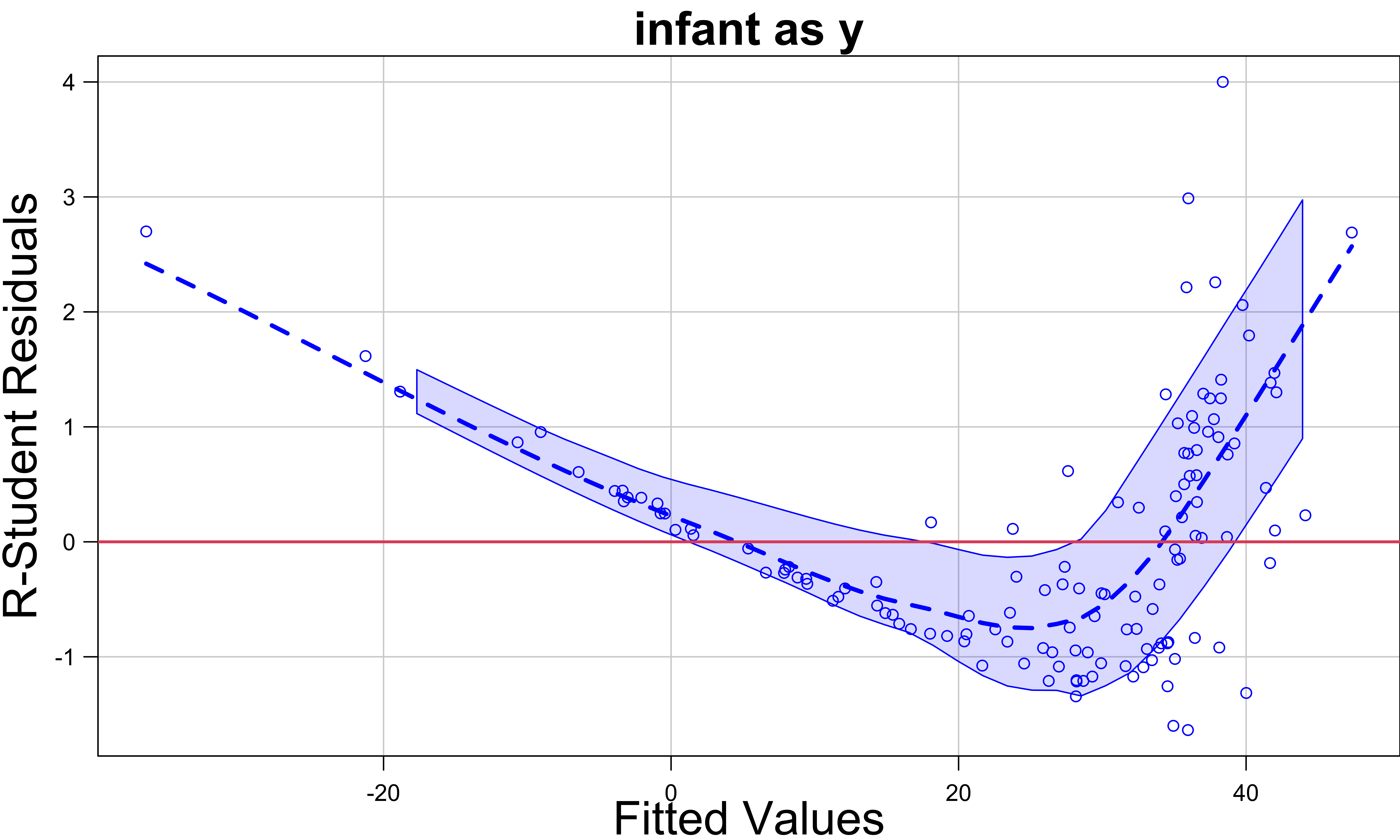
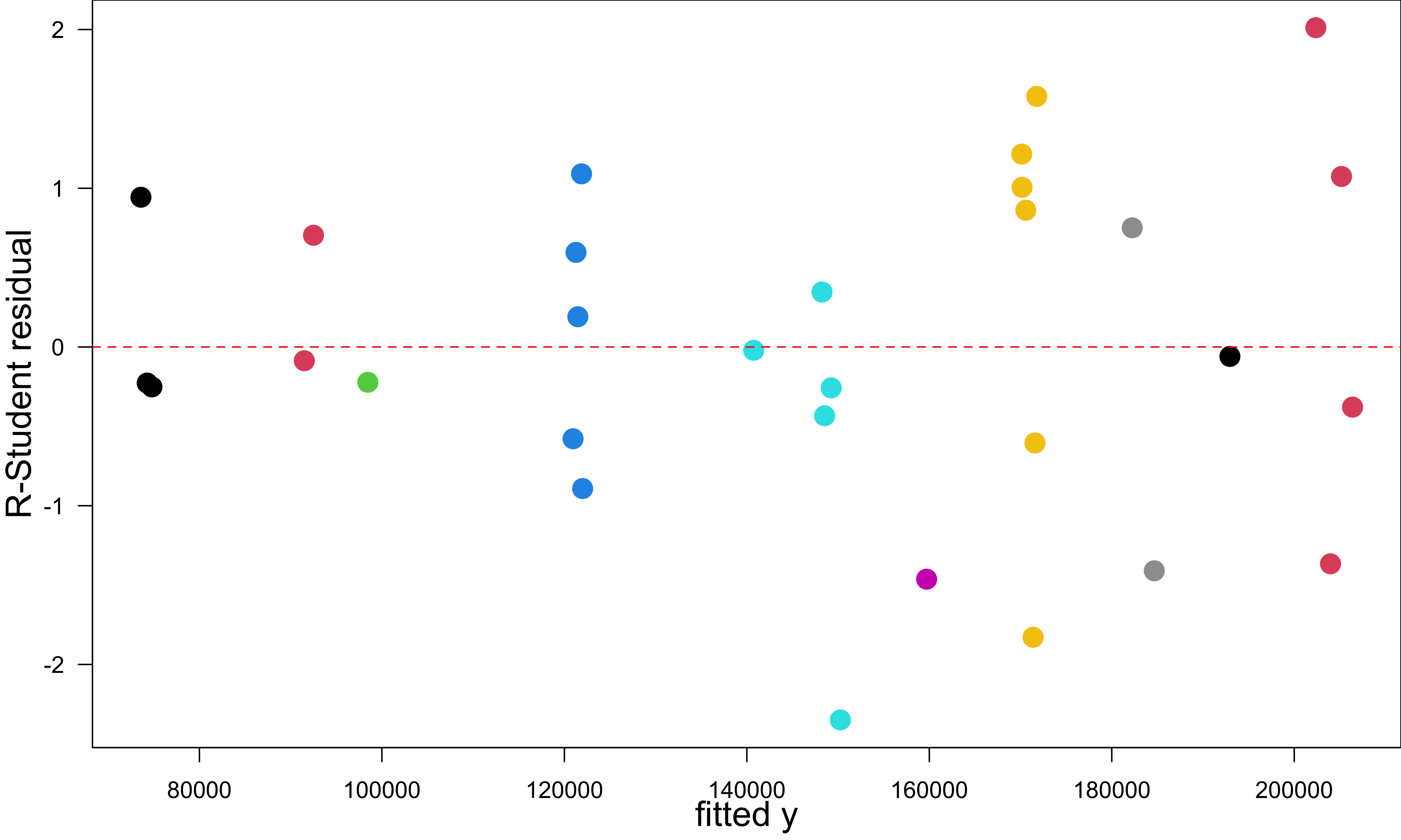
• The residuals increase with fitted values.

• Nonlinear pattern.

• Nonsense negative fitted values.

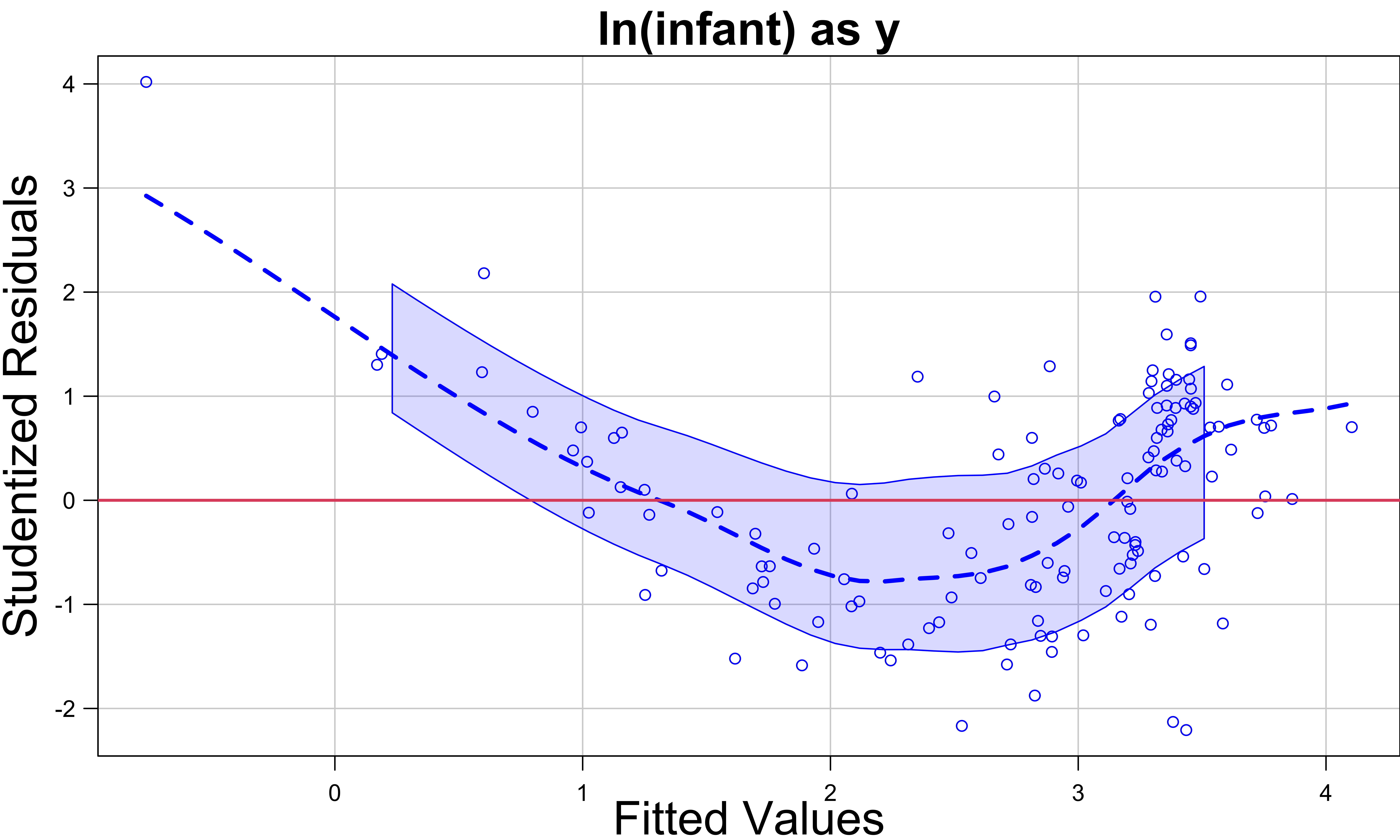
• Variation around the central smooth seems approximately constant.

• Nonlinearity is still apparent. (Linearity and lack of fit next week)

• The nonlinear pattern suggests there are serious problems of the linear model.

• The residuals increases with fitted values.

• Several nonsense negative fitted values.

residual plot can reveal nonlinearity, but can;t determine where the problem lies and how to correct it.

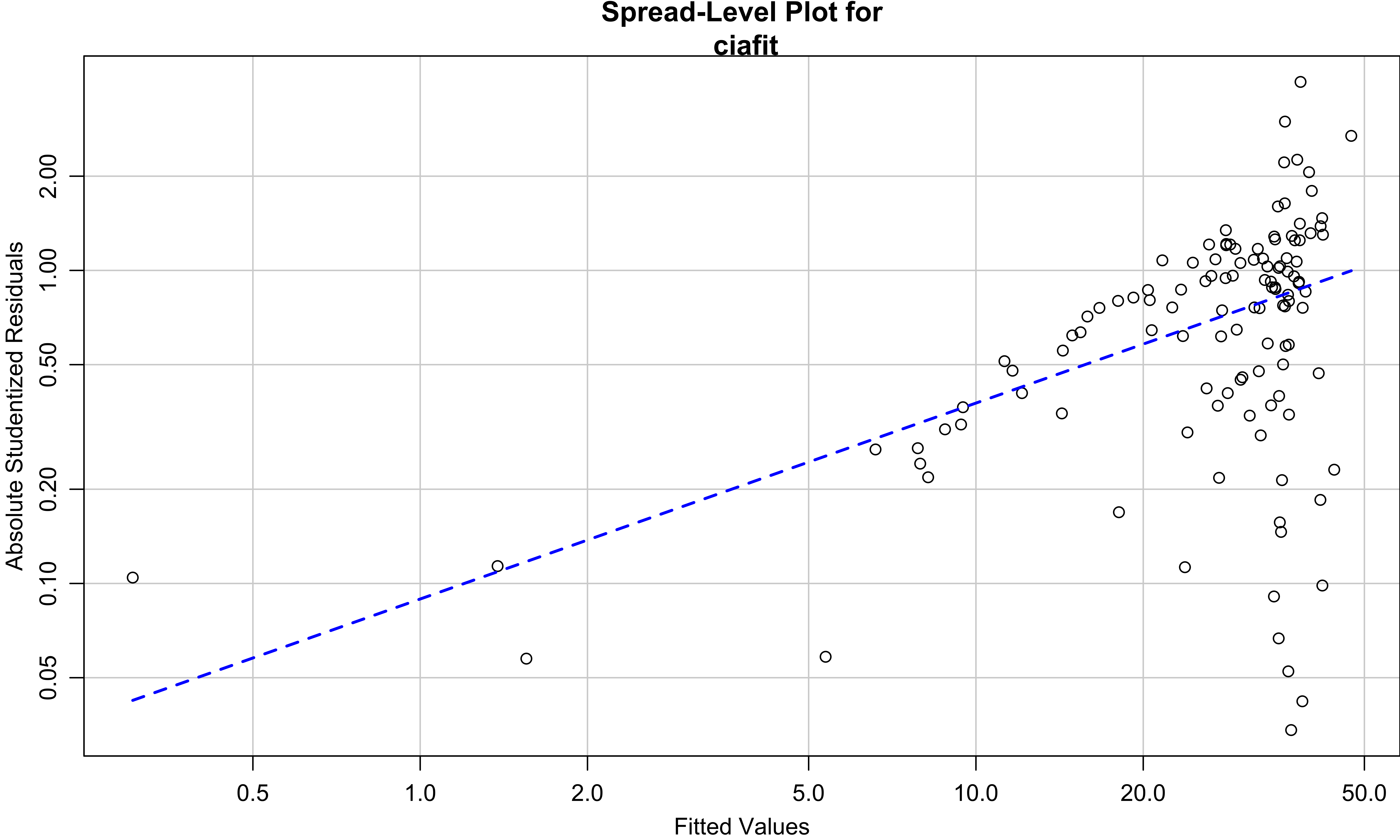
Tukey’s Spread-Level Plot

• Plot log of the absolute R-Student residuals vs. log of the (positive) fitted values.
• The fitted line slope \(b\) suggests a variance-stablizing power transformation \(\lambda = 1 - b\) for \(y\).

car::spreadLevelPlot(ciafit, smooth = FALSE)

Suggested power transformation:  0.37 

spreadLevelPlot(logciafit, smooth = FALSE)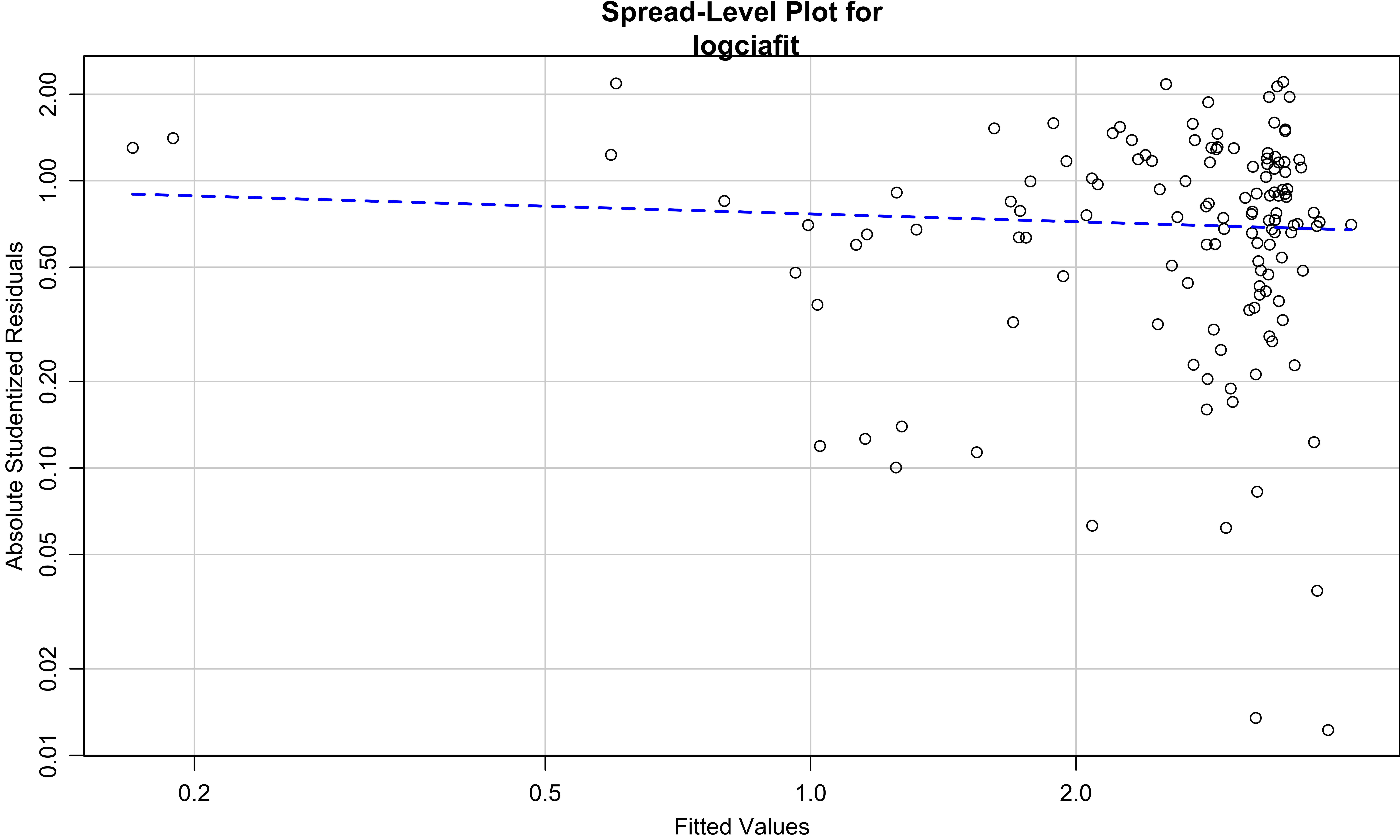

Suggested power transformation:  1.1 

• Plot log of the absolute R-Student residuals vs. log of the (positive) fitted values

• Fit by robust regression to generate fitted lines.

• The slope \(b\) of the fitted line suggests a variance-stablizing power transformation \(\lambda = 1 - b\) for \(y\).

Weighted Least Squares (WLS)

• Suppose that the other assumptions hold but that the error variances differ: \(\epsilon_i \stackrel{indep}{\sim} N(0, \sigma_i^2)\)

• The resulting model isn’t estimable because we have more parameters than data points.

• If we know the pattern of unequal error variances, so that \(\sigma_i^2 = \sigma^2/w_i\), for known values \(w_i\), we can compute the coefficient estimates that minimize the Weighted Residual Sum of Squares.

• In simple linear regression, \[S(\beta_0, \beta_1) = \sum_{i=1}^nw_i\epsilon_i^2 = \sum_{i=1}^n w_i \left(y_i - \beta_0 - \beta_1x_i \right)^2\]

Observations with large variances will have smaller weights.

\[(b_0, b_1, \dots, b_k) = \underset{{\beta_0, \beta_1, \dots, \beta_k}}{\mathrm{arg \, min}} S(\beta_0, \beta_1, \dots, \beta_k)\]

\[S(\beta_0, \beta_1, \dots, \beta_k) = \sum_{i=1}^nw_i\epsilon_i^2 = \sum_{i=1}^nw_i\left(y_i - \beta_0 - \sum_{j=1}^k\beta_j x_{ij}\right)^2\]

Methods of Choosing Weights

• Prior knowledge or information

• Residual analysis

  • \(\mathrm{Var}(\epsilon_i) \propto x_{i}\), suggest \(w_i = 1/x_{i}\)
  • When \(y_i\) is an average of \(n_i\) observations at \(x_i\), \(\mathrm{Var}(y_i) =\sigma^2 / n_{i}\) and suggest \(w_i = n_i\)

• Chosen inversely proportional to variances of measurement error

.alert[ If we have no idea of \(\bf W\), consider feasible GLS estimator \(\hat{\bsbeta}_{FGLS} = {\bf(X'\hat{W}X)^{-1}X'\hat{W}y}\), where \(\bf \hat{W}\) is an estimate of \(\bf W\) from some method. ] - The weights, \(w_i\), or in general \(\bf V\) must be known. - Prior knowledge or information - Residual analysis + \(\mathrm{Var}(\epsilon_i) \propto x_{i}\), suggest \(w_i = 1/x_{i}\) + When \(y_i\) is an average of \(n_i\) observations at \(x_i\), \(\mathrm{Var}(y_i) =\sigma^2 / n_{i}\) and suggest \(w_i = n_i\) - Chosen inversely proportional to variances of measurement error - Guess at the weights and iteratively estimate them.

R Lab Example 5.5 Food Sales in LRA

• The average monthly revenue vs. annual advertising expenses for 30 restaurants.

Code

x <- c(3000, 3150, 3085, 5225, 5350, 6090, 8925, 9015, 8885, 8950, 9000, 11345,
       12275, 12400, 12525, 12310, 13700, 15000, 15175, 14995, 15050, 15200,
       15150, 16800, 16500, 17830, 19500, 19200, 19000, 19350)
y <- c(81464, 72661, 72344, 90743, 98588, 96507, 126574, 114133, 115814, 123181,
       131434, 140564, 151352, 146926, 130963, 144630, 147041, 179021, 166200, 180732,
       178187, 185304, 155931, 172579, 188851, 192424, 203112, 192482, 218715, 214317)
group <- c(1, 1, 1, 2, 2, 3, 4, 4, 4, 4, 4, 5, 5, 5, 5, 5, 6, 7, 7, 7, 7, 7, 7, 
           8, 8, 9, 10, 10, 10, 10)
ex5_5 <- data.frame("expense" = x, "sales" = y, "group" = group)
par(mar = c(3.3, 3.3, 0, 0), mgp = c(2, 1, 0))
plot(ex5_5$expense, ex5_5$sales, xlab = "Advertising expense", 
     ylab = "Food sales", col = group, pch = 16, cex = 2, cex.lab = 1.5)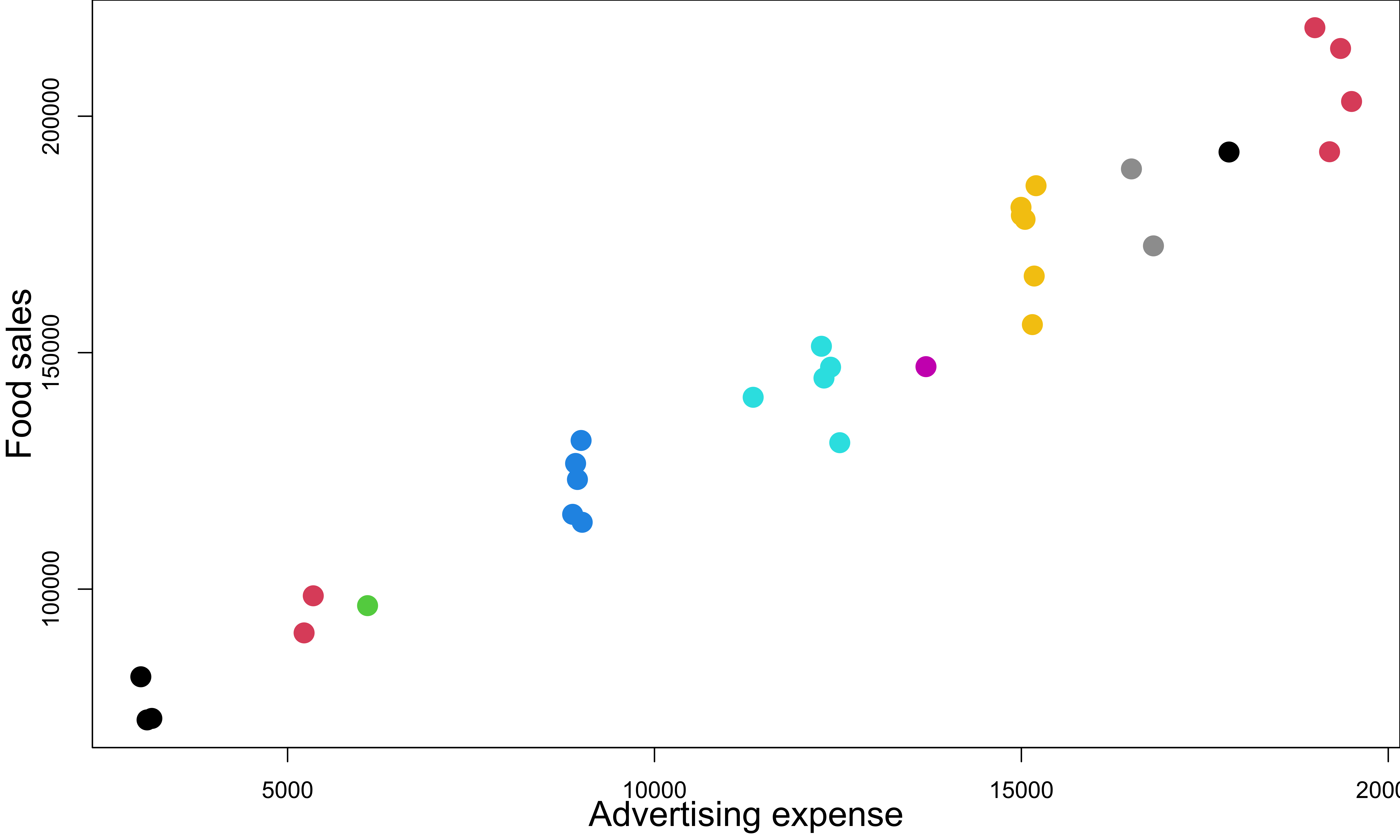

• The average monthly income from food sales vs. annual advertising expenses for 30 restaurants.
• Management is interested in the relationship between these variables.

R Lab Non-constant Variance

• \(\hat{y} = 49443.384 + 8.048x\)

R Lab Determine Weights

• There are several sets of \(x\) values that are “near neighbors”.

ex5_5$expense

 [1]  3000  3150  3085  5225  5350  6090  8925  9015  8885  8950  9000 11345
[13] 12275 12400 12525 12310 13700 15000 15175 14995 15050 15200 15150 16800
[25] 16500 17830 19500 19200 19000 19350

ex5_5$group

 [1]  1  1  1  2  2  3  4  4  4  4  4  5  5  5  5  5  6  7  7  7  7  7  7  8  8
[26]  9 10 10 10 10

• Assume that these near neighbors are close enough to be considered repeat points.
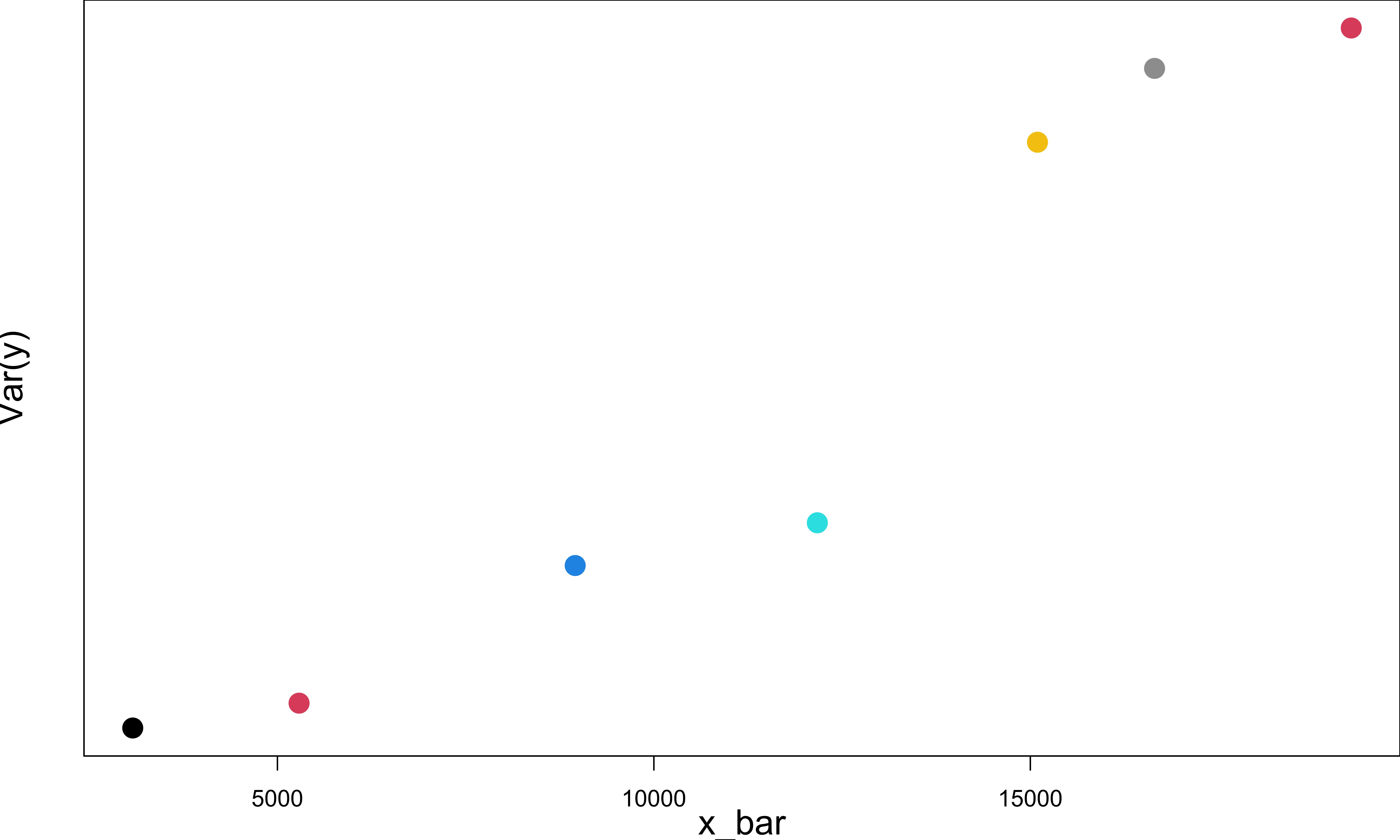
• Use the variance of the responses at those repeat points to investigate how \(\mathrm{Var}(y)\) changes with \(x.\)

R Lab Determine Weights

• The empirical variance of \(y\), \(s_y^2\), increases approximately linearly with \(\bar{x}\).

R Lab Determine Weights

• \(\hat{s}^2_y = -9226002 + 7781.6\bar{x}\)
• Substituting each \(x_i\) value into this equation will give an estimate of the variance of the corresponding observation \(y_i\), \(\hat{s}^2_i\)
• The inverse of these \(\hat{s}^2_i\) will be reasonable estimates of the weights \(w_i\).

s2_fit <- lm(s2_y~x_bar)
(coef <- s2_fit$coef)

(Intercept)       x_bar 
   -9226002        7782 

s2_i <- coef[1] + coef[2] * ex5_5$expense
(wt <- 1 / s2_i)

 [1] 7.1e-08 6.5e-08 6.8e-08 3.2e-08 3.1e-08 2.6e-08 1.7e-08 1.6e-08 1.7e-08
[10] 1.7e-08 1.6e-08 1.3e-08 1.2e-08 1.1e-08 1.1e-08 1.2e-08 1.0e-08 9.3e-09
[19] 9.2e-09 9.3e-09 9.3e-09 9.2e-09 9.2e-09 8.2e-09 8.4e-09 7.7e-09 7.0e-09
[28] 7.1e-09 7.2e-09 7.1e-09

R Lab WLS fit

(wls_fit <- lm(ex5_5$sales ~ ex5_5$expense, 
               weights = wt))

...
Coefficients:
  (Intercept)  ex5_5$expense  
     51024.81           7.92  
...

• \(\hat{y} = 51024.8 + 7.918x\)
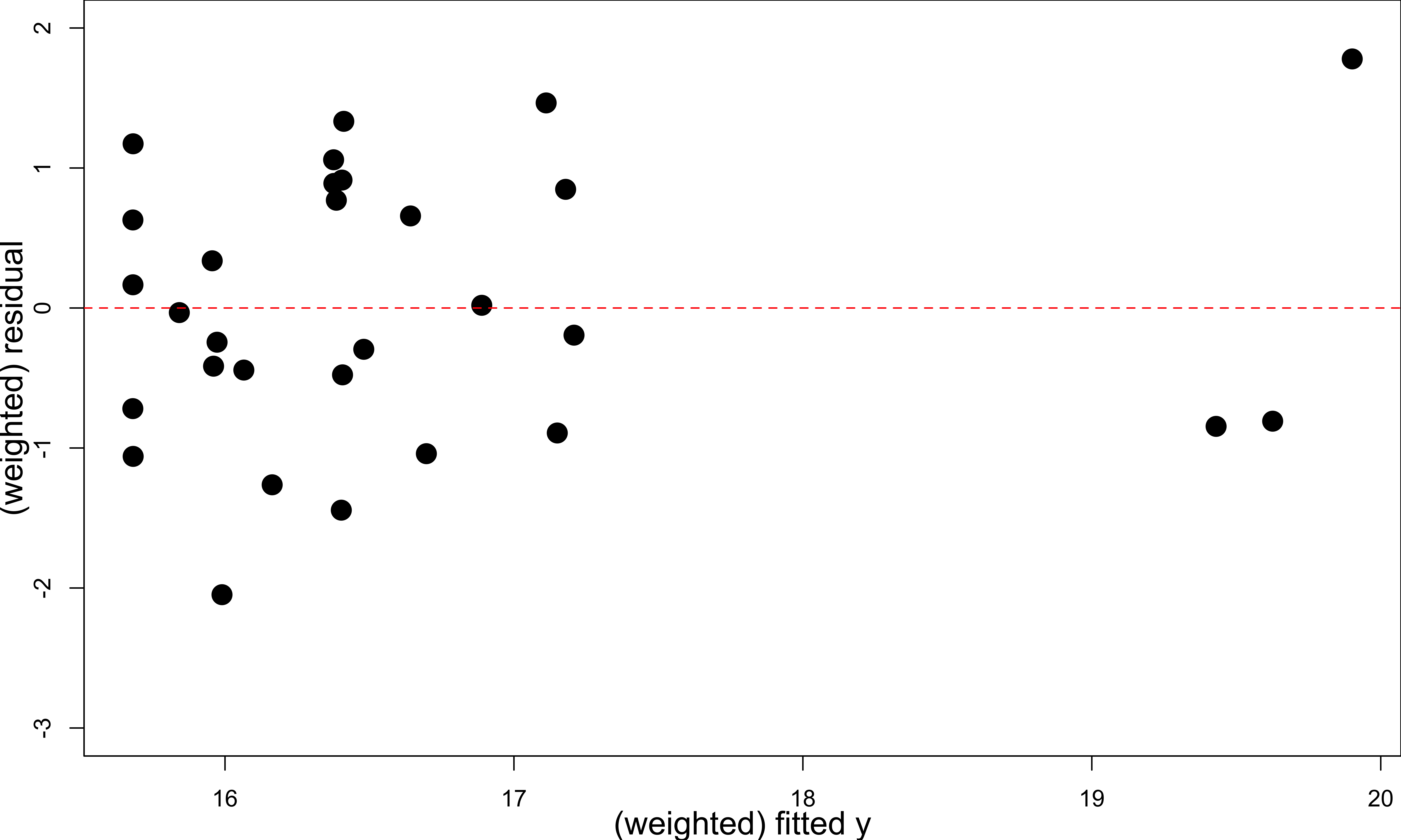
• We must examine the residuals to determine if using WLS has improved the fit.
• Plot the weighted residuals \(w_i^{1/2}(y_i - \hat{y}_i^W)\), where \(\hat{y}_i^W\) comes form the WLS fit, against \(w_i^{1/2}\hat{y}_i^W\)

.alert[ The WLS residuals and the WLS fitted values when the model assumes \(\mathrm{Var}(\boldsymbol \epsilon) = \sigma^2 {\bf W}^{-1}\) should behave as the OLS residuals and OLS fitted values when the model assumes \(\mathrm{Var}(\boldsymbol \epsilon) = \sigma^2 {\bf I}\).

R Lab WLS Residual Plot

• The residual plot has no significant fanning.