Regression Diagnostics: Normality 📖

MATH 4780 / MSSC 5780 Regression Analysis

Dr. Cheng-Han Yu
Department of Mathematical and Statistical Sciences
Marquette University

Assumptions of Linear Regression

\(Y_i= \beta_0 + \beta_1X_{i1} + \beta_2X_{i2} + \dots + \beta_kX_{ik} + \epsilon_i\)

• \(E(Y \mid X)\) and \(X\) are linearly related.
• \(\small E(\epsilon_i) = 0\)
• \(\small \mathrm{Var}(\epsilon_i) = \sigma^2\)
• \(\small \mathrm{Cov}(\epsilon_i, \epsilon_j) = 0\) for all \(i \ne j\).
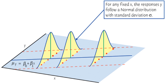
• \(\small \epsilon_i \stackrel{iid}{\sim} N(0, \sigma^2)\) (for statistical inference)

• So it’s not that uncommon to see violation of assumptions.
• Today, we are going to learn how to check whether those assumptions are valid or satisfied.
• And probably the following two weeks, if the assumptions are not satisfied, how do we deal with it. OK.

• If the assumptions are violated, a different sample could lead to a different conclusion!
• \(R^2\) tells us how good the model is fitted to the data, but says nothing about the correctness of the model.
• All the inferences are based on the assumption that the model is correct.

Model Adequacy Checking and Correction

Non-normality

Non-constant Error Variance

Non-linearity and Lack of Fit

• This week we are going to learn some methods to correct model inadequacy.
• We can either transform our data, our use a more general method, called Generalized Least Squares or Weighted Least Squares.
• \(\epsilon_i \stackrel{iid}{\sim} N(0, \sigma^2)\): mean 0, constant variance, normally distributed, and uncorrelated.
• \(E(\epsilon_i) =0\) implies the function form of the model (linearity) is correct.

Non-normality

• The central limit theorem assures the validity of inferences based on the least-squares (LS) coefficients in all but small samples.

Without normality,

• Heavier tailed errors:
  • LS estimators do not have the smallest variance among unbiased estimators.
  • give rise to outliers.

Gauss-Markov does not require normality.

• Skewed errors:
  • tend to generate outliers in the direction of the skew.
  • the conditional mean of \(y\) given \(x\) is not a good measure of center of a highly skewed distribution.

• Multimodal errors:
  • suggest the omission of one or more categorical regressors.

• \(\epsilon_i \stackrel{iid}{\sim} N(0, \sigma^2)\): mean 0, constant variance, normally distributed, and uncorrelated.
• The form of the model (linearity) and the specification of the predictors are correct.
• Check model adequacy by residual plots and lack-of-fit tests.
• Methods for building models when some of the assumptions are violated.
  • data transformation
  • generalized least squares (GLS) and weighted least squares (WLS)

Detecting Nonnormality

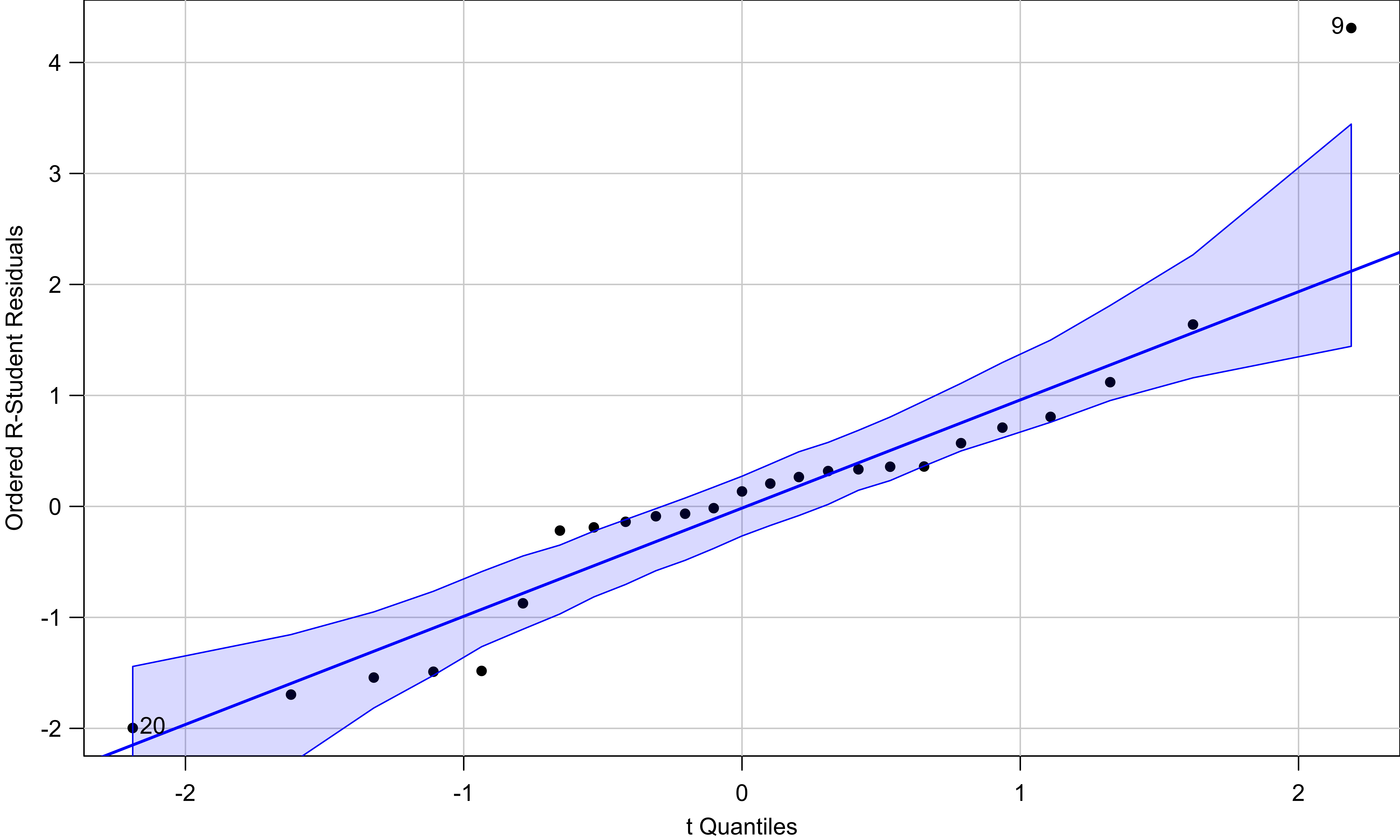
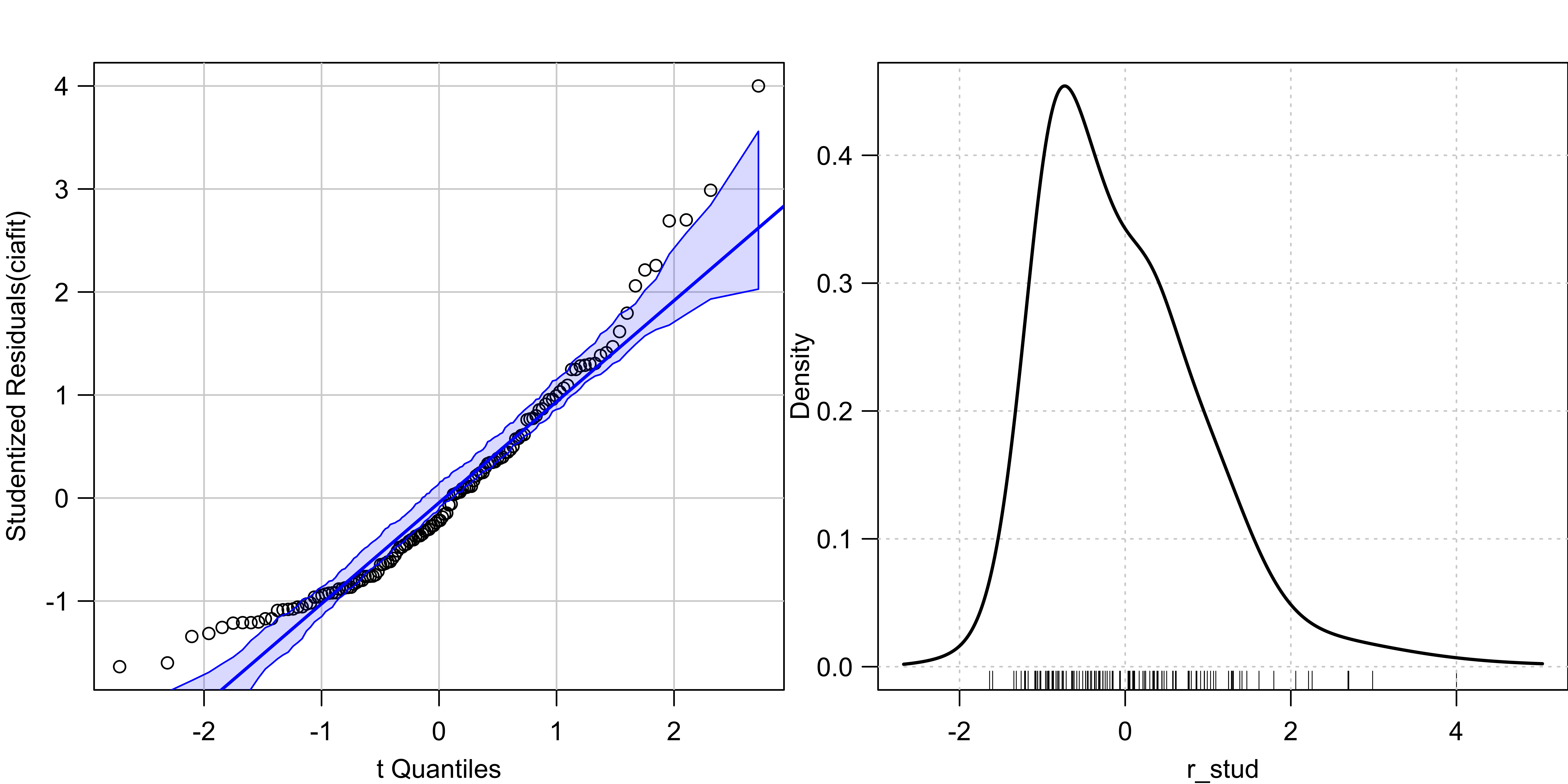
• The R-student residuals \(t_i \sim t_{n-p-1}\) if the model assumptions are correct.

• Compare the distribution of the \(t_i\)s to \(t_{n-p-1}\) in QQ plot.

• One way to address the assumption of normality is to compare the distribution of the R-student residuals to \(t_{n-p-1}\) in QQ plot.

QQ plot of R-Student Residuals Comparing \(t_{n-p-1}\)

car::qqPlot(delivery_lm, id = TRUE, col.lines = "blue", 
            reps = 1000, ylab = "Ordered R-Student Residuals", pch = 16)

• The car package calls the R-student residuals studentized residuals.
• if put lm object, car::qqPlot automatically create qqplot for R-student residual comparing with \(t_{n-p-1}\) distribution.
• No severe problem in delivery data
• id = controls point identification; if FALSE, no points are identified; can be a list of named arguments to the showLabels function; TRUE is equivalent to list(method=“y”, n=2, cex=1, col=carPalette()[1], location=“lr”), which identifies the 2 points with the 2 points with the most extreme verical values — studentized residuals for the “lm” method.

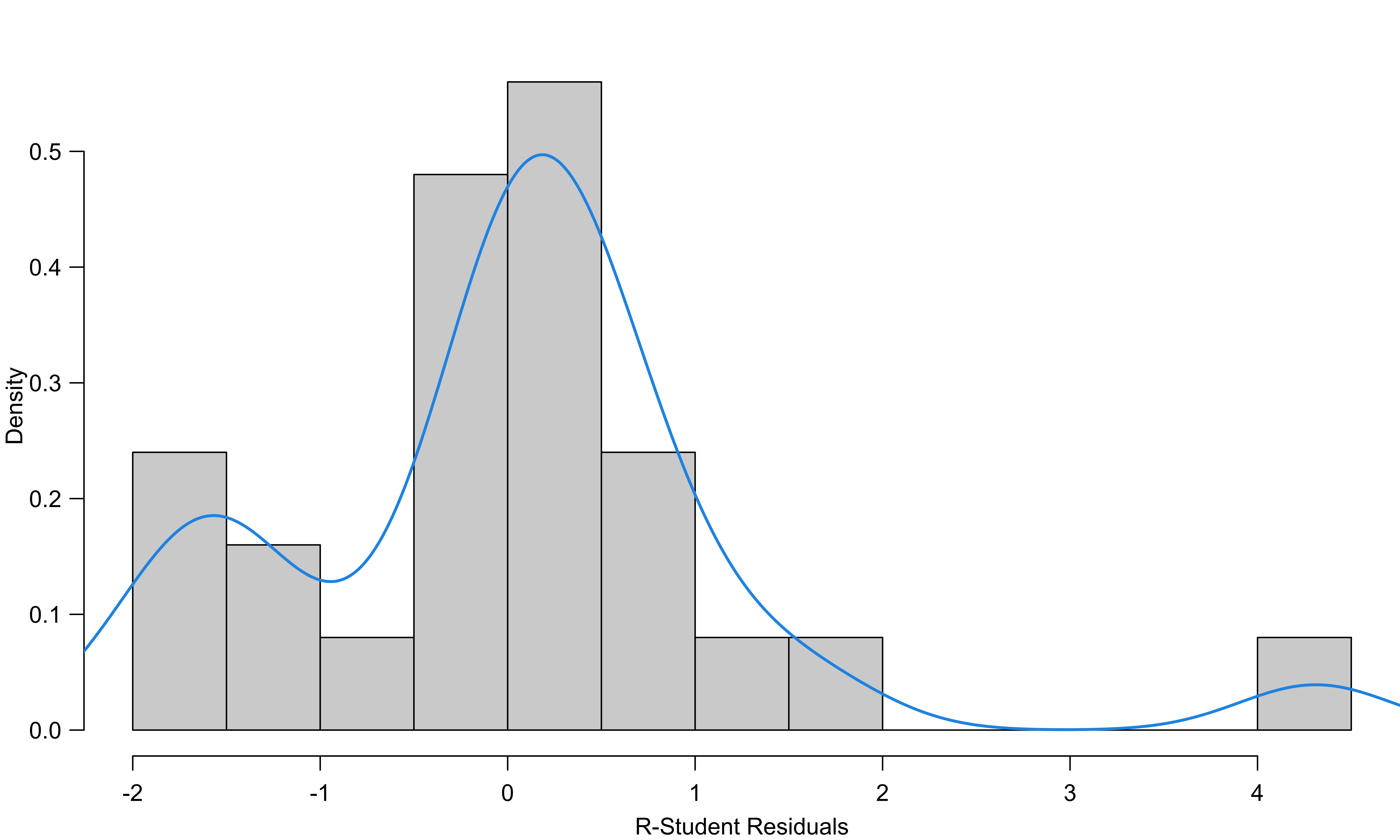
Density plot of R-Student Residuals

rstud <- rstudent(delivery_lm)
hist(rstud, prob = TRUE, breaks = 10, xlab = "R-Student Residuals", main = "")
lines(density(rstud, adjust = 2), col = 4, lwd = 2)

• The QQ plot draws attention to the tail behavior of the R-student residuals but is less effective in visualizing their distribution as a whole.
• Check histogram or smooth density plot of the R-student residuals to get the general shape of the distribution.
• May be better to add another categorical regressor
• car::densityPlot(rstud, adjust = 2, xlab = “R-Student Residuals”)

Correcting Nonnormality

• A response that is close to normal usually makes the assumption of normal errors more tenable.

• Heavier tailed errors:

  • Use robust regression (Chap 15 in LRA)

• Skewed errors:

  • Transform response data for symmetry

• Multimodal errors:

  • Add one or more relevant categorical variables.

Want the error or the response conditional on \(x\)s to be like normal after correction.

Transformation for Symmetry

Power transformation: \(y \rightarrow y^{\lambda}\)

• make the distribution of \(y\) more normal, at least more symmetric.
• \(y\) can take on positive values only.
• \(y \rightarrow \ln(y)\) for \(\lambda = 0.\)

Ladder of powers and roots (Tukey, 1977):

• No transformation: \(\lambda = 1\)
• Descending: spreads out the small values of \(y\) relative to the large values.
  • \(\lambda = 1/2\) (square root); \(\lambda = 0\) (natural log); \(\lambda = -1\) (inverse)
• Ascending: spreads out the large values relative to the small values.
  • \(\lambda = 2\) (square); \(\lambda = 3\) (cube)

if \(\lambda\) is descending from \(1\) to \(-1\), the fransformation increasingly spreads out the small values of \(y\) relative to the large values.

The order of \(y\) is reversed if \(\lambda < 0\) is used for power transformation.

Correcting Skewness by Power Transformation

Box-Cox Transformation on \(y\)

A modified power transformation by Box and Cox (1964):

\[y^{(\lambda)} = \begin{cases} \frac{y^{\lambda}-1}{\lambda}, & \quad \lambda \ne 0\\ \ln y, & \quad \lambda = 0 \end{cases}\]

• For all \(\lambda\), \(y^{(\lambda)} = 1\) at \(y = 1\).
• The order of the transformed data \(y^{(\lambda)}\) is the same as that of \(y\), even for \(\lambda < 0.\)

• The derivative w.r.t. \(y\) of \(y^{(\lambda)}\) at \(y = 1\) is 1 for any \(\lambda\).

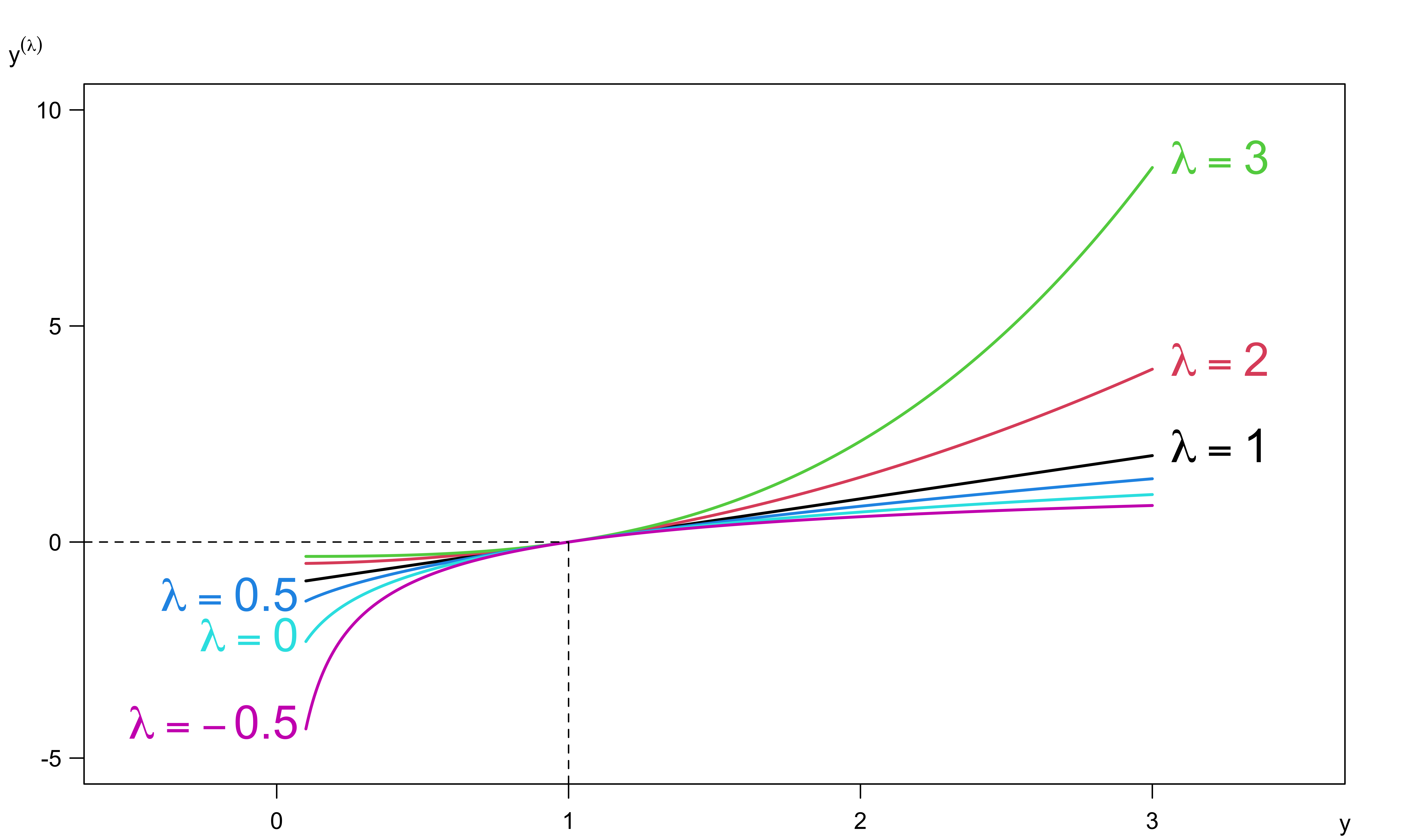
Box-Cox Transformation on \(y\): Choose \(\lambda\) Analytically

• The model to be fit is \[y_i^{(\lambda)} = \beta_0 + \beta_1x_{i1}+ \cdots + \beta_kx_{ik} + \epsilon_i^*\]
• Choose \(\lambda\) so that the transformed errors \(\epsilon_i^*\) look as nearly normally distributed as possible.

R Lab CIA World Factbook Data

            gdp infant gini health  region
Albania    11.1   12.8   34    6.0  Europe
Algeria    14.3   21.0   35    5.2  Africa
Argentina  22.1    9.7   46    8.5 America
Armenia     7.4   13.5   31    4.5  Europe
Australia  46.6    4.4   30    9.1 Oceania
Austria    45.4    3.5   26   11.5  Europe
Azerbaijan 17.9   25.7   34    5.4    Asia
Bangladesh  3.4   44.1   32    3.6    Asia
Belarus    18.2    3.6   27    5.0  Europe
Belgium    41.7    3.4   26   10.8  Europe
Benin       1.9   55.7   36    4.5  Africa
Bhutan      7.7   35.9   39    3.8    Asia

• gdp: GDP per capita in thousands of U.S. dollars
• infant: Infant mortality rate per 1000 live births
• gini: Gini coefficient for the distribution of family income
• health: Health expenditures as a percentage of GDP

R Lab R-Student Residuals

• See how gdp, health and gini affect infant.
• R-Student residuals are right-skewed, suggesting transforming the response, infant mortality, down the ladder of powers.

ciafit <- lm(infant ~ gdp + health + gini, data = CIA)
r_stud <- rstudent(ciafit)
car::qqPlot(ciafit, id = FALSE)
car::densityPlot(r_stud)

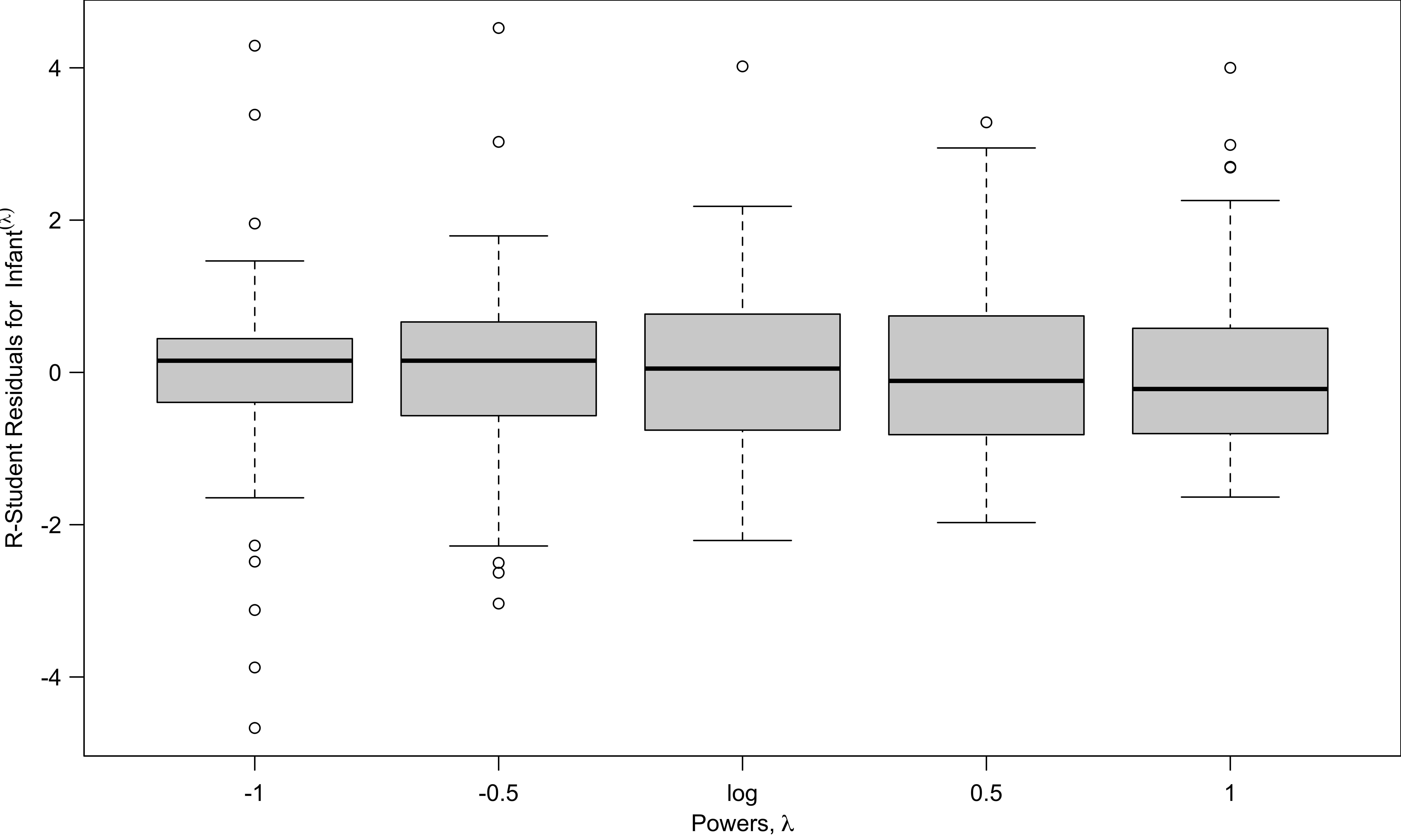
R Lab Box-Cox Transformation

Code

mat <- matrix(r_stud)
for (lam in c(0.5, 0, -0.5, -1)) {
    refit <- update(
        ciafit, car::bcPower(infant, lam) ~ .
        )
    mat <- cbind(rstudent(refit), mat)
}
colnames(mat) <- c(-1, -0.5, "log", 0.5, 1)
boxplot(
    mat, id = FALSE, 
    xlab = expression("Powers," ~ lambda),
    ylab = expression(
        "R-Student Residuals for " 
        ~ Infant ^ (lambda))
    )

R Lab Choose \(\lambda\) Analytically

summary(car::powerTransform(ciafit, family = "bcPower"))

bcPower Transformation to Normality 
   Est Power Rounded Pwr Wald Lwr Bnd Wald Upr Bnd
Y1     -0.22       -0.33        -0.37       -0.072

Likelihood ratio test that transformation parameter is equal to 0
 (log transformation)
                      LRT df  pval
LR test, lambda = (0)   8  1 0.005

Likelihood ratio test that no transformation is needed
                      LRT df   pval
LR test, lambda = (1) 181  1 <2e-16

• \(\hat{\lambda} = -0.22\), and the \(95\%\) CI for \(\lambda\) is \([-0.37, -0.07]\).
• \(\lambda = 1\) not in the interval, providing support for transforming response.
• \(\lambda = 0\) (log transformation) is slightly outside the interval.

car::powerTransform() uses the maximum likelihood-like approach to select a \(\lambda\) estimate, \(\hat{\lambda}\).

Other Issues

• Apply power transformations to data with zero or negative values by adding a positive constant to the data to make all values positive.
  • \(\log(y + 10)\) if all \(y > -10\).

• Power transformations are effective when the ratio of the largest to smallest values is sufficiently large.
  • If \(y_{max}/y_{min} \approx 1\), power transformations are nearly linear.
  • Increase the ratio by adding a negative constant, \((y_{max} - c)/(y_{min}-c)\)

• If acceptable, choose log transformation for simple interpretation.

logciafit <- lm(log(infant) ~ gdp + health + gini, data = CIA)
coef(logciafit)

(Intercept)         gdp      health        gini 
      3.016      -0.044      -0.055       0.022 

• All else held constant, for one unit increase of gdp, the infant mortality rate is expected to be decreased, on average, by 4.3% because \(\exp(-0.044) = 0.957\).

Hawkins and Weisberg (2017) - Skewed conditional distribution of \(y\) is not a good measure of center. + Create a model for conditional median of the response. (Quantile regression) - OLS regression of the original variable is used to to estimate the expected arithmetic mean and OLS regression of the log transformed outcome variable is to estimated the expected geometric mean of the original variable.