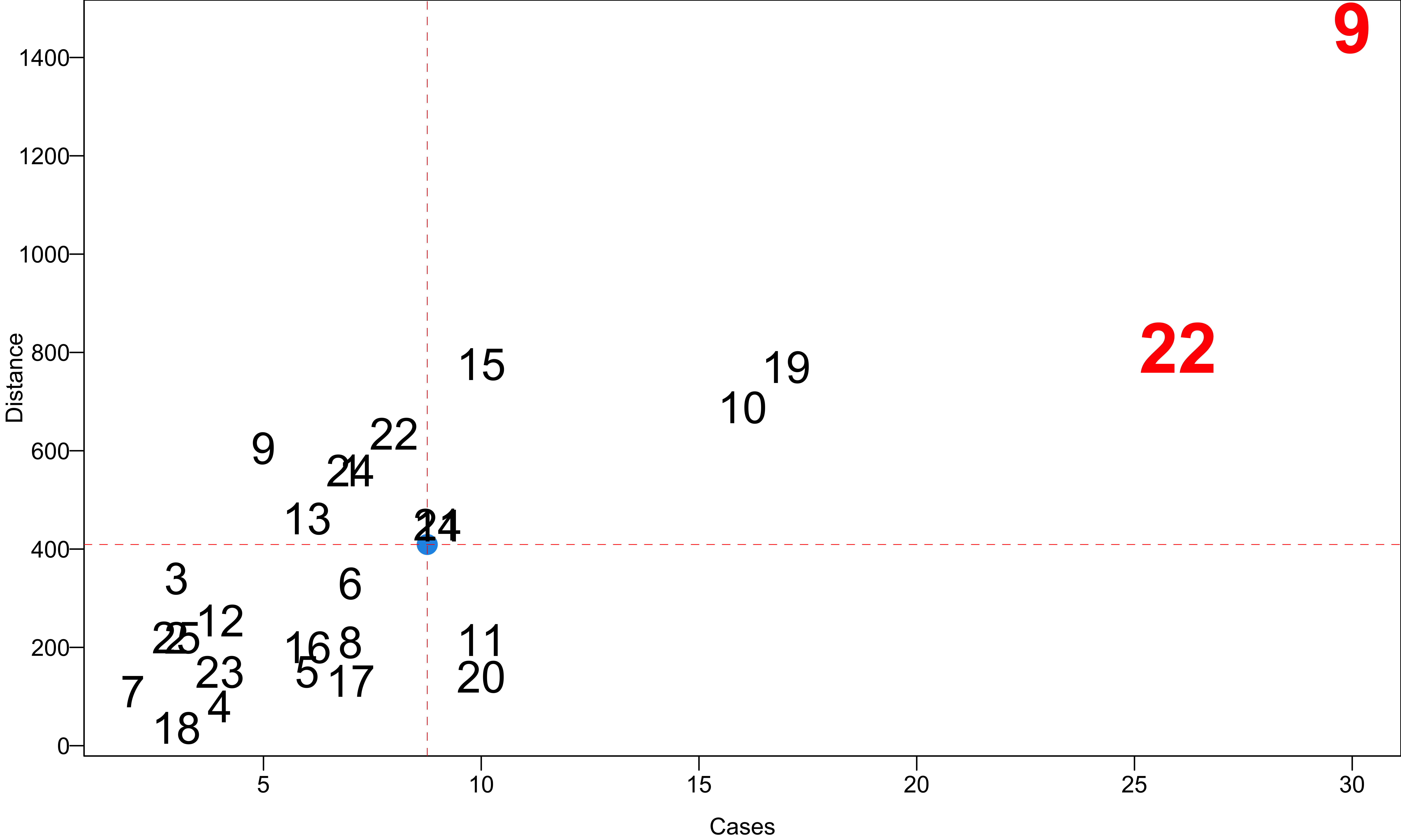
   time cases distance
1  16.7     7      560
2  11.5     3      220
3  12.0     3      340
4  14.9     4       80
5  13.8     6      150
6  18.1     7      330
7   8.0     2      110
8  17.8     7      210
9  79.2    30     1460
10 21.5     5      605
11 40.3    16      688
12 21.0    10      215
13 13.5     4      255
14 19.8     6      462
15 24.0     9      448
16 29.0    10      776
17 15.3     6      200
18 19.0     7      132
19  9.5     3       36
20 35.1    17      770
21 17.9    10      140
22 52.3    26      810
23 18.8     9      450
24 19.8     8      635
25 10.8 4 150Regression Diagnostics: Unusual Data 👩💻
MATH 4780 / MSSC 5780 Regression Analysis
Department of Mathematical and Statistical Sciences
Marquette University
Unusual Data
Outliers
Leverage
Influence
Outliers: Unusual \(y\)
- An outlier is a case whose response value is unusual given the value of the regressors.
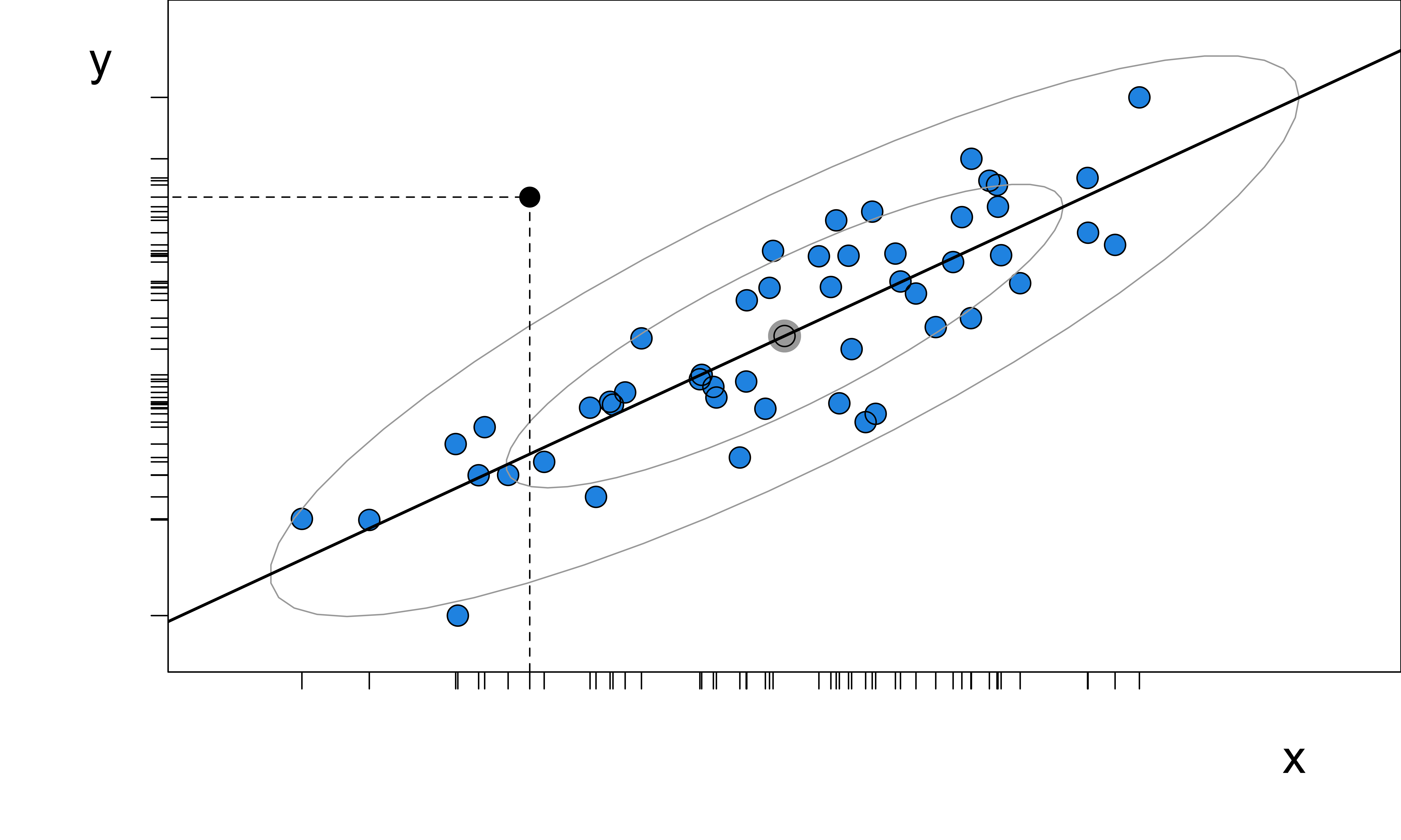
Leverage: Unusual \(x\)
- Points that are away from the center of the data cloud of \({\bf x}\) are called leverage points.
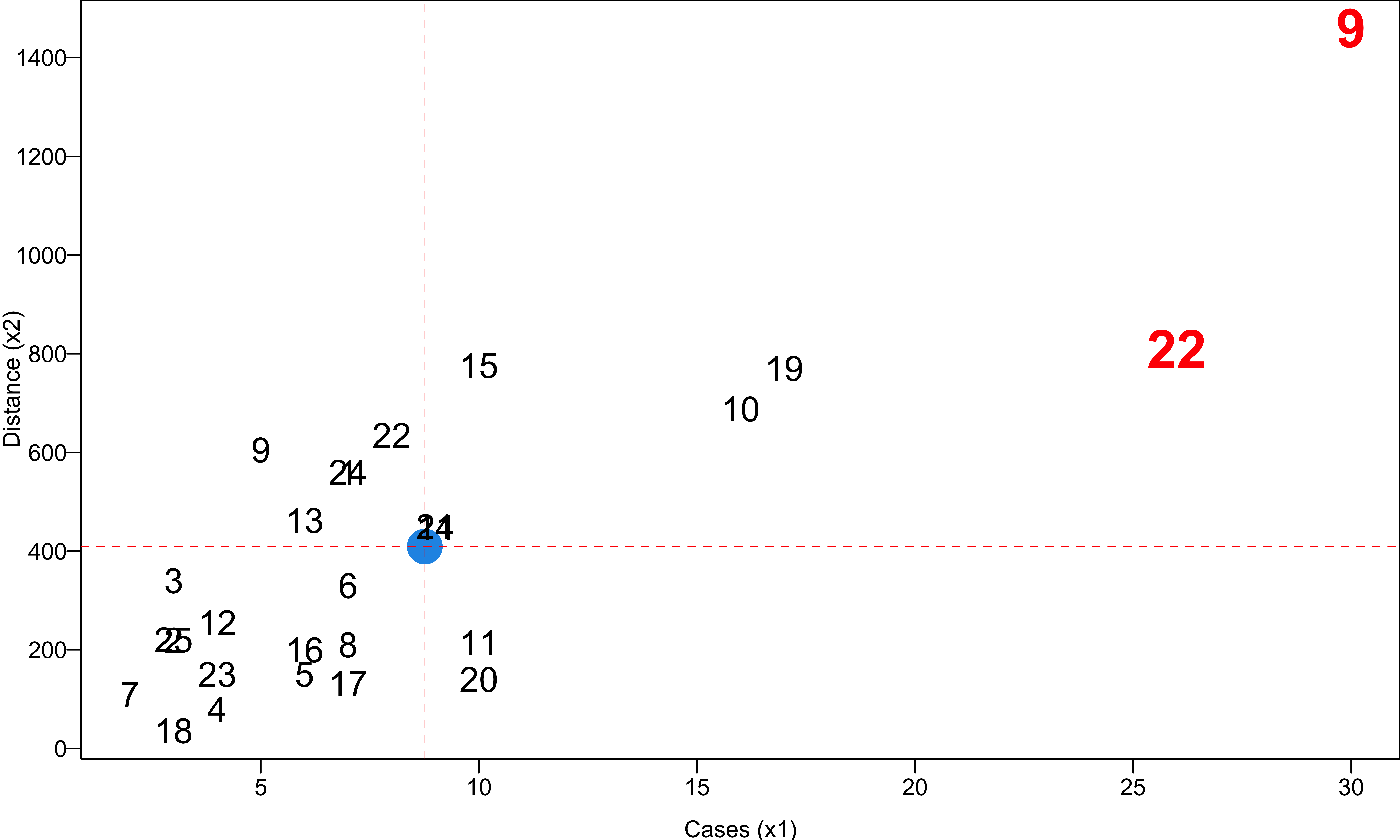
Observation 9 and 22 are away from the center of \({\bf x}\) space, and are likely leverage points.
Influence: Unusual \(x\) and \(y\)
- An influential point has great influence on estimated regression coefficients. \[\text{Influence} = \text{Leverage} \times \text{Outlyingness}\]
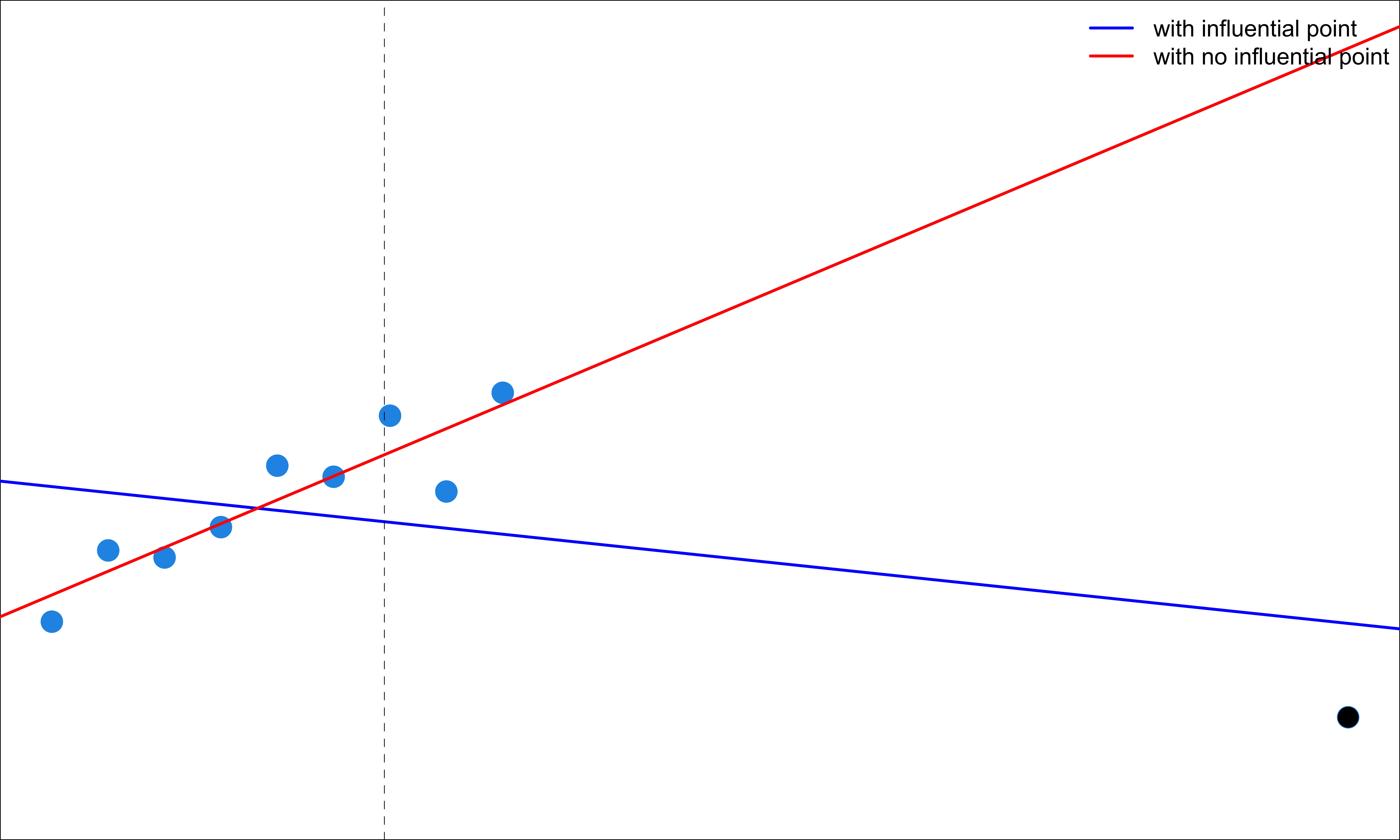
Unusual Data: Outliers, Leverage and Influence
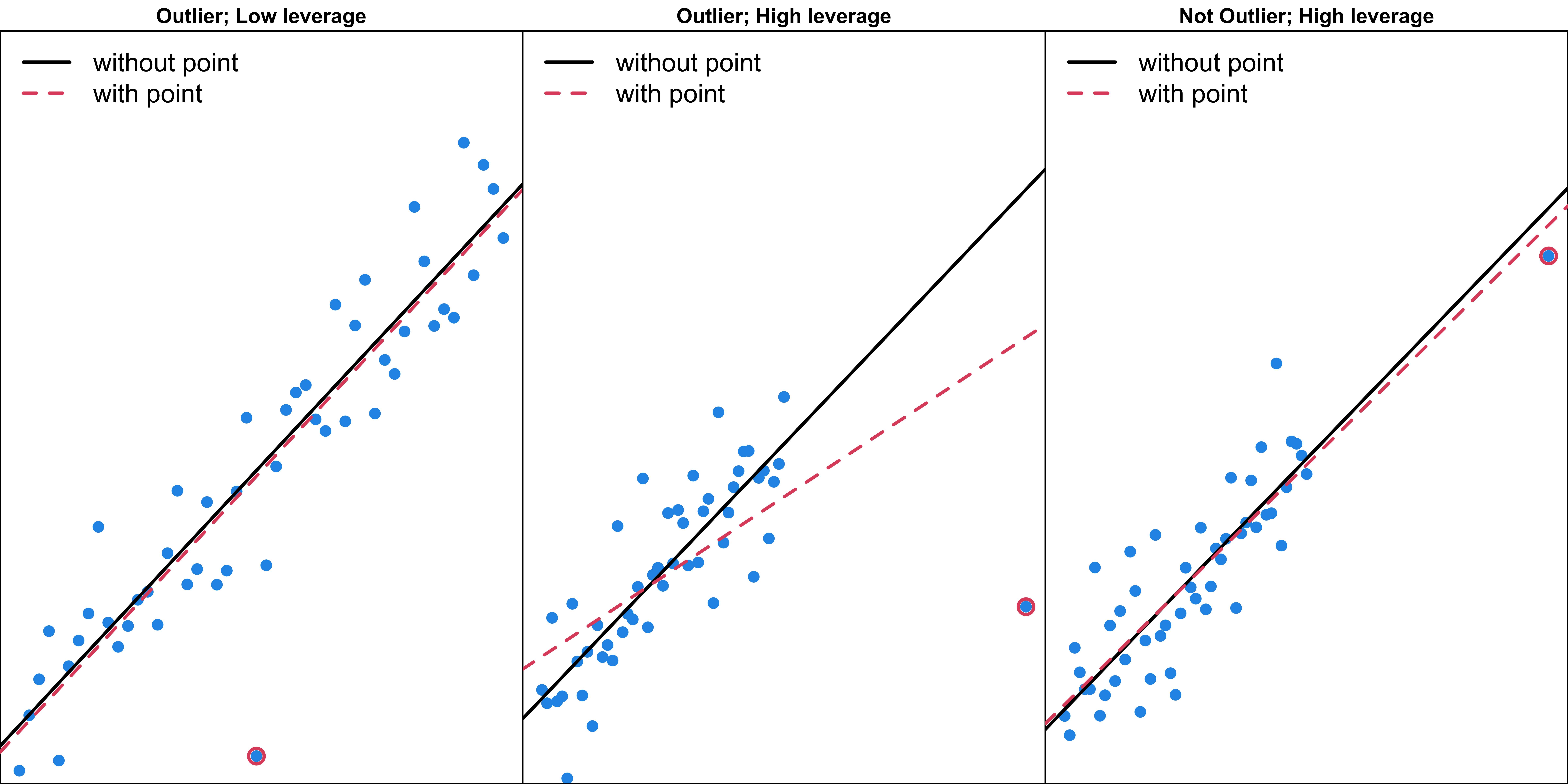
Measuring Leverage: Hat Values
\({\bf H} = {\bf X(X'X)}^{-1} {\bf X}'\).
The hat value \(h_{ii}\) is the \(i\)th diagonal element of \(\bf H\).
\(h_{ii} \in \left[\frac{1}{n}, 1\right]\) is a standardized measure of the distance of the \(i\)th case from the centroid of the \(\bf x\) space, taking into account the correlational structure of the \(x\)s.
The larger the \(h_{ii}\) is, the farther the point \({\bf x}_i\) lies to the centroid of the \(\bf x\) space.
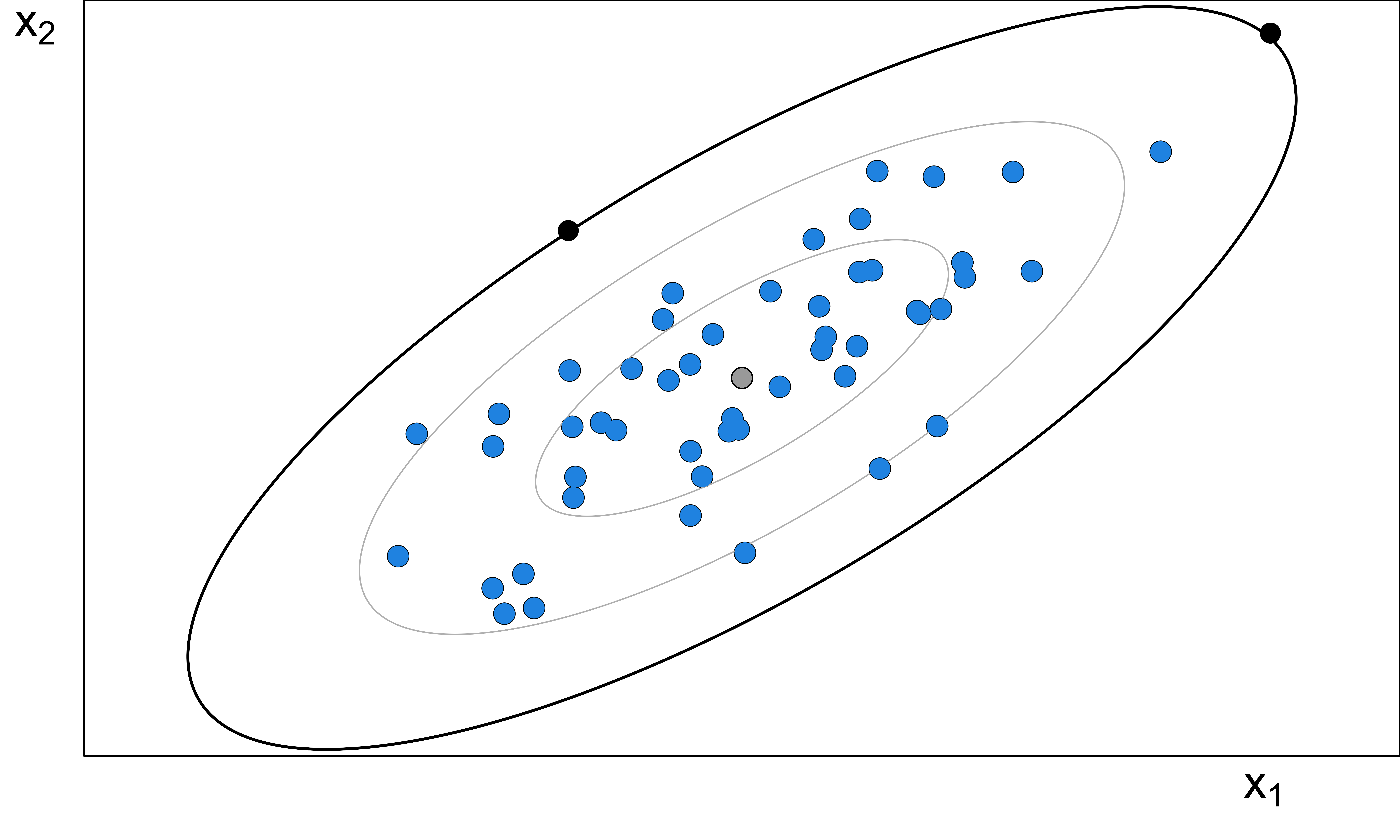
Measuring Leverage: Hat Values
In simple linear regression, \[h_{ii} = \frac{1}{n} + \frac{\left(x_i - \bar{x}\right)^2}{S_{xx}}\]
\(\hat{y}_j = b_0 + b_1 ~x_j = h_{j1}y_1 + h_{j2}y_2 + \cdots + h_{jn}y_n\)
\(h_{ii} = \sum_{j=1}^nh_{ji}^2\) summarizes the influence (the leverage) of \(y_i\) on all the fitted values \(\hat{y}_j\), \(j = 1, \dots, n\).
\(\bar{h} = \frac{\sum_{i=1}^n h_{ii}}{n} = p/n\)
A point with \(h_{ii} > 2\bar{h}\) is considered a leverage point.
R Lab Delivery Time Leverage Points
    9    22    10    16    21    24    12     1    20     3    19    18    11
0.498 0.392 0.196 0.166 0.165 0.121 0.114 0.102 0.102 0.099 0.096 0.096 0.086
    4     7    14     5     2    25     8    13    17     6    23    15
0.085 0.082 0.078 0.075 0.071 0.067 0.064 0.061 0.059 0.043 0.041 0.041 Detecting Outliers
Measure the conditional unusualness of \(y\) given \({\bf x}\).
❌ Can’t just use residual \(e_i\) to measure the unusualness of \(y_i\)!
If the point is also a leverage point (large \(h_{ii}\)), it’s residual tends to be small.
- R-student residual: \[t_i = \frac{e_i}{\sqrt{s^2_{(i)}(1-h_{ii})}}\] where \(s^2_{(i)}\) estimates \(\sigma^2\) based on the data with the \(i\)th point removed.
- \(t_i \sim t_{n-p-1}\) and a formal testing procedure can be used for detecting outliers.
- A point with \(|t_i| > 2\) needs to be examined with care.
R Lab Detecting Outliers - Residual Plot
    9     4    18    10    11    19     8     2    14    13     7    15    17
 4.31  1.64  1.12  0.81  0.71  0.57  0.36  0.36  0.33  0.32  0.26  0.21  0.13
    3    25     6     5    12    16    21    23    22    24     1    20
-0.02 -0.07 -0.09 -0.14 -0.19 -0.22 -0.87 -1.48 -1.49 -1.54 -1.70 -2.00 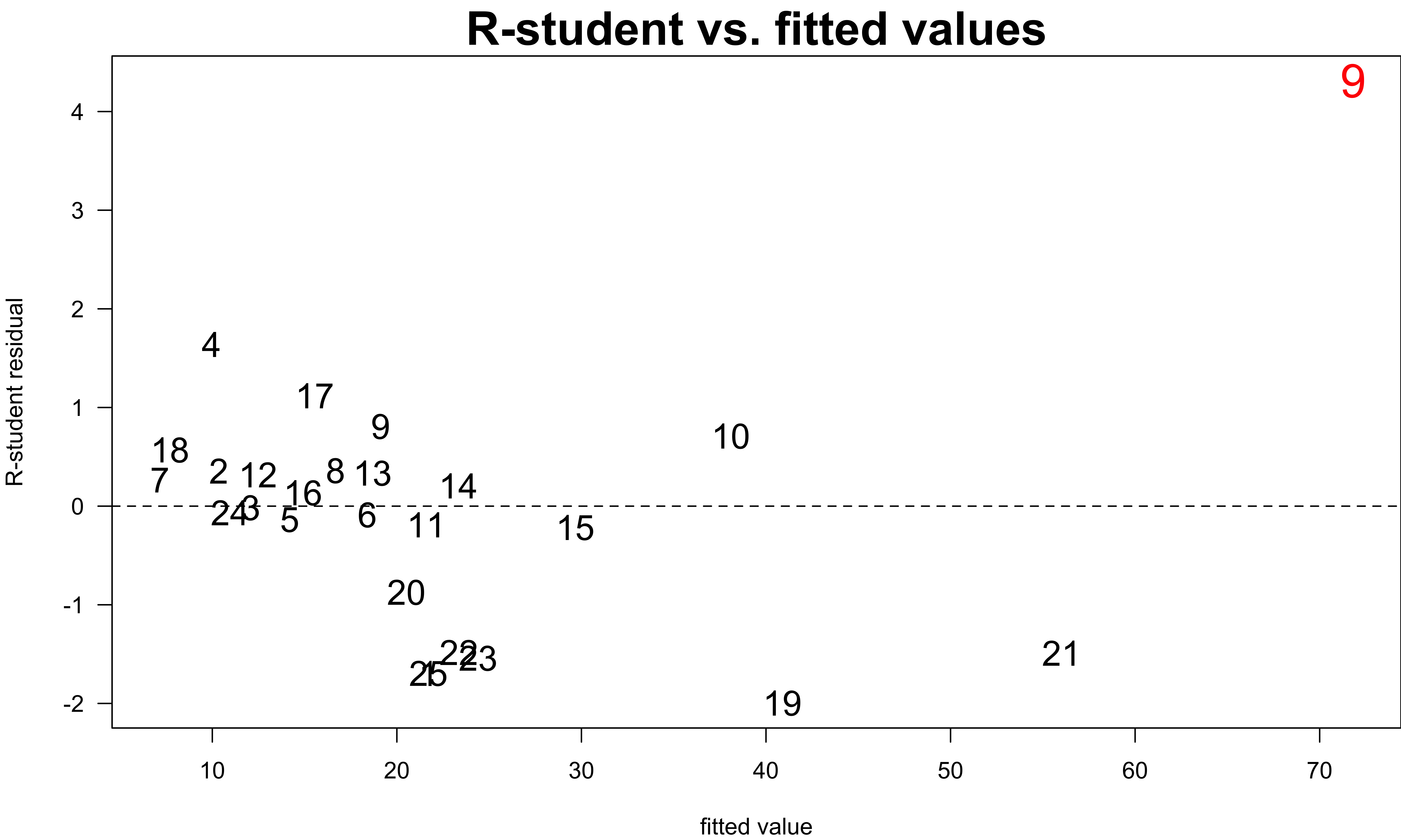
Measuring Influence
- The influence measures are those that measure the effect of deleting the \(i\)th observation.
- \(DFBETAS_{j, i}\) measures the effect on coefficient \({b_j}\) when the \(i\)th observation is removed.
- Cook’s Distance \(D_i\) measures the effect of the \(i\)th observation on coefficient vector \({\bf b}\).
- \(DFFITS_{i}\) measures the effect on fitted value \(\hat{y}_i\).
- \(COVRATIO_{i}\) measures the effect on the precision of estimates (variance).
\(DFBETAS_{j, i}\)
- \(DFBETAS_{j, i}\) measures how much the regression coefficient \(b_j\) changes in standard error units if the \(i\)th observation is removed. \[DFBETAS_{j, i} = \frac{b_j - b_{j(i)}}{\sqrt{s_{(i)}^2C_{jj}}} = \frac{b_j - b_{j(i)}}{se_{(i)}(b_j)}\] where
- \(b_{j(i)}\) is the \(j\)th coefficient estimate computed without the \(i\)th observation.
- \(C_{jj}\) is the diagonal element of \(( {\bf X}'{\bf X})^{-1}\) corresponding to \(b_j\).
- The \(i\)th point is considered influential on \(j\)th coefficient if \(|DFBETAS_{j, i}| > 2/\sqrt{n}\).
- One issue: there are \(np\) DFBETAS measures.
R Lab \(DFBETAS_{j, i}\)
   (Intercept) cases distance
1        -0.19  0.41    -0.43
2         0.09 -0.05     0.01
3         0.00  0.00     0.00
4         0.45  0.09    -0.27
5        -0.03 -0.01     0.02
6        -0.01  0.00     0.00
7         0.08 -0.02    -0.01
8         0.07  0.03    -0.05
9        -2.58  0.93     1.51
10        0.11 -0.34     0.34
11       -0.03  0.09     0.00
12       -0.03 -0.05     0.05
13        0.07 -0.04     0.01
14        0.05 -0.07     0.06
15        0.02  0.00     0.01
16        0.00  0.06    -0.08
17        0.03  0.01    -0.02
18        0.25  0.19    -0.27
19        0.17  0.02    -0.10
20        0.17 -0.21    -0.09
21       -0.16 -0.30     0.34
22        0.40 -1.03     0.57
23       -0.16  0.04    -0.05
24       -0.12  0.40    -0.47
25 -0.02 0.00 0.01- Point 9 is influential, as its deletion results in a displacement of every coefficient by at least 0.9 standard deviation of \(b_j\).
Cook’s Distance \(D_i\)
- \(D_i\) measures the squared distance that the vector of fitted values moves when the \(i\)th observation is deleted.
\[D_i = \frac{(\hat{{\bf y}}_{(i)} - \hat{{\bf y}})'(\hat{{\bf y}}_{(i)}-\hat{{\bf y}})}{p s^2} = \frac{r_i^2}{p}\frac{h_{ii}}{1-h_{ii}}, \quad i = 1, 2, \dots, n\] where \(r_i = \frac{e_i}{\sqrt{s^2(1-h_{ii})}}\) is the Studentized residuals.
- What contributes to \(D_i\):
- How well the model fits the \(i\)th observation (larger \(r_i^2\) for poorer fit)
- How far the point is away from the remaining data (larger \(h_{ii}\) for higher leverage)
- \(\text{Influence} = \text{Leverage} \times \text{Outlyingness}\)
Consider points with \(D_{i} > 1\) to be influential.
R Lab Cook’s Distance \(D_i\)
  9
3.4 9 22 20 24 1 4 10 21 18 23 11 19 2
3.419 0.451 0.132 0.102 0.100 0.078 0.054 0.051 0.044 0.030 0.016 0.012 0.003
14 16 8 13 7 12 15 5 17 6 25 3
0.003 0.003 0.003 0.002 0.002 0.002 0.001 0.001 0.000 0.000 0.000 0.000 - Observation 9 is influential using the cutoff of one, and the point 22 is not.
\(D_i > 1\) may risk missing unusual data. Use \(4/(n-p)\) instead.
\(DFFITS_{i}\)
- \(DFFITS_{i}\) measures the influence of the \(i\)th observation on the \(i\)th fitted value, again in standard deviation units. \[DFFITS_{i} := \frac{\hat{y}_i - \hat{y}_{(i)}}{\sqrt{s_{(i)}^2h_{ii}}} = \left(\frac{h_{ii}}{1-h_{ii}}\right)^{1/2}t_i\] where \(\hat{y}_{(i)}\) is the fitted value of \(y_i\) computed without the \(i\)th observation.
- The denominator provides a standardization since \(\mathrm{Var}\left( \hat{y}_i\right) = \sigma^2h_{ii}\).
- \(DFFITS_{i}\)is essentially the R-student residual scaled by the leverage \([h_{ii}/(1-h_{ii})]^{1/2}\).
A point with \(|DFFITS_{i}| > 2\sqrt{p/n}\) needs attention.
R Lab \(DFFITS_{i}\)
    1     2     3     4     5     6     7     8     9    10    11    12    13
-0.57  0.10 -0.01  0.50 -0.04 -0.02  0.08  0.09  4.30  0.40  0.22 -0.07  0.08
   14    15    16    17    18    19    20    21    22    23    24    25
0.10 0.04 -0.10 0.03 0.37 0.19 -0.67 -0.39 -1.20 -0.31 -0.57 -0.02 9 22
4.3 -1.2 - Deleting point 9 displaces the predicted response \(\hat{y}_{(i)}\) by over four standard deviations of \(\hat{y}_i.\)
\(COVRATIO_{i}\)
\(DFFITS_{i}\) and \(DFBETAS_{j, i}\) reflect influence on \(\hat{y}_i\) and \(b_j\), but do not indicate whether or not the presence of the \(i\)th point appreciably sharpened the estimation of the coefficient.
A scalar measure of precision, called generalized variance of \({\bf b}\) is \[GV({\bf b}) = \det\left( \mathrm{Cov}({\bf b}) \right) = \det\left( \sigma^2 ({\bf X'X})^{-1} \right) \]
-
To express the role of the \(i\)th observation on the precision of estimation, we use \[COVRATIO_{i} = \frac{ \det \left( \left( {\bf X}_{(i)}' {\bf X}_{(i)} \right)^{-1} s_{(i)}^2 \right) }{\det \left( \left( {\bf X'X} \right)^{-1} s^2\right)} = \frac{ \left( s_{(i)}^2 \right)^p}{\left( s^2 \right) ^ p}\left( \frac{1}{1-h_{ii}}\right)\]
- \({\bf X}_{(i)}\) denotes the \((n-1) \times p\) data matrix with the \(i\)th observation eliminated.
\(COVRATIO_{i}\)
\[\small COVRATIO_{i} = \frac{ \det \left( \left( {\bf X}_{(i)}' {\bf X}_{(i)} \right)^{-1} s_{(i)}^2 \right) }{\det \left( \left( {\bf X'X} \right)^{-1} s^2 \right)} = \frac{ \left( s_{(i)}^2 \right)^p}{\left( s^2 \right) ^ p}\left( \frac{1}{1-h_{ii}}\right)\]
If \(COVRATIO_{i} > 1\), the \(i\)th case improves the precision.
If \(COVRATIO_{i} < 1\), the \(i\)th case degrades the precision.
Higher leverage \(h_{ii}\) leads to larger \(COVRATIO_{i}\) and improves the precision unless the point is an outlier in \(y\) space.
If \(i\)th point is an outlier, \(\frac{s_{(i)}^2}{s^2} < 1\).
Cutoffs:
- \(COVRATIO_{i} > 1 + 3p/n\) or
- \(COVRATIO_{i} < 1 - 3p/n\) provided that \(n > 3p\).
R Lab \(COVRATIO_{i}\)
   1    2    3    4    5    6    7    8    9   10   11   12   13   14   15   16
0.87 1.21 1.28 0.88 1.24 1.20 1.24 1.21 0.34 1.31 1.17 1.29 1.21 1.23 1.19 1.37
  17   18   19   20   21   22   23   24   25
1.22 1.07 1.22 0.76 1.24 1.40 0.89 0.95 1.23 16 22
1.4 1.4 9
0.34 Since \(COVRATIO_{9} < 1\), this observation degrades precision of estimation.
Since \(COVRATIO_{22} > 1\), this observation tends to improve precision of estimation.
Point 22 and 16 barely exceed the cutoff, so their influence is small.
Jointly Influential Points
- Subset of cases can be jointly influential or can offset each other’s influence.
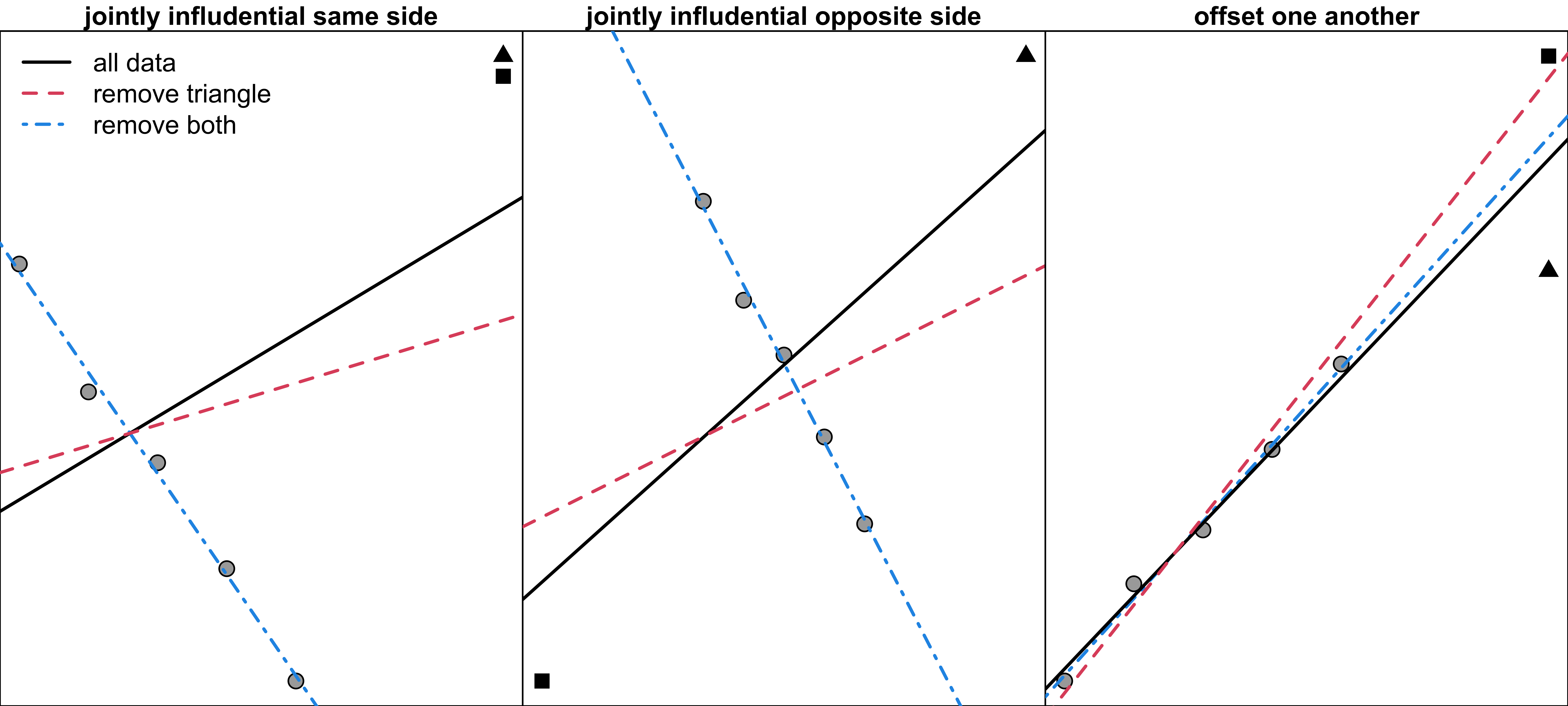
Detecting Joint Influence: Added-Variable Plot
- \(y_i= \beta_0 + \beta_1x_{i1} + \beta_2x_{i2} + \dots + \beta_kx_{ik} + \epsilon_i\).
To create the added-variable plot for \(x_1\),
- Step 1: Regress \(y\) on all predictors except \(x_1\) and obtain residuals \[\small \begin{align}\hat{y}_i(x_{(1)}) &= b_0^{(1)} + b_2^{(1)}x_{i2} + \dots + b_k^{(1)}x_{ik}\\e_i(y \mid x_{(1)}) &= y_i - \hat{y}_i(x_{(1)}) \end{align}\]
- Step 2: Regress \(x_1\) on all other predictors and obtain residuals \[\small \begin{align}\hat{x}_{i1}(x_{(1)}) &= a_0^{(1)} + a_2^{(1)}x_{i2} + \dots + a_k^{(1)}x_{ik}\\e_i(x_1 \mid x_{(1)}) &= x_{i1} - \hat{x}_{i1}(x_{(1)}) \end{align}\]
- Step 3: Plot \(e_i(y \mid x_{(1)})\) vs. \(e_i(x_1 \mid x_{(1)}), \quad i = 1, \dots, n\)
- For any \(x_j\), \(e_i(y \mid x_{(j)})\) vs. \(e_i(x_j \mid x_{(j)})\)
R Lab Duncan’s Occupational Prestige Data
                   type income education prestige
plumber              bc     44        25       29
chemist            prof     64        86       90
gas.stn.attendant    bc     15        29       10
store.manager      prof     42        44       45
teacher            prof     48        91       73
insurance.agent      wc     55        71       41
bookkeeper           wc     29        72       39
author             prof     55        90       76
electrician          bc     47        39       53
lawyer             prof     76        98       89
policeman            bc     34        47       41
mail.carrier         wc     48        55       34
soda.clerk           bc     12        30        6
machinist            bc     36        32       57
banker             prof     78        82       92
streetcar.motorman bc 42 26 19-
type: Type of occupation-
prof(professional and managerial) -
wc(white-collar) -
bc(blue-collar)
-
income: Percentage who earned $3,500 or more per yeareducation: Percentage who were high school graduatesprestige: Percentage of respondents in a survey who rated the occupation as “good” or better in prestige
R Lab Added-Valued Plot
- The slope of the least square simple regression line of \(e_i(y \mid x_{(1)})\) on \(e_i(x_1 \mid x_{(1)})\) is the same as the slope \(b_1\) for \(x_1\) in the full multiple regression.
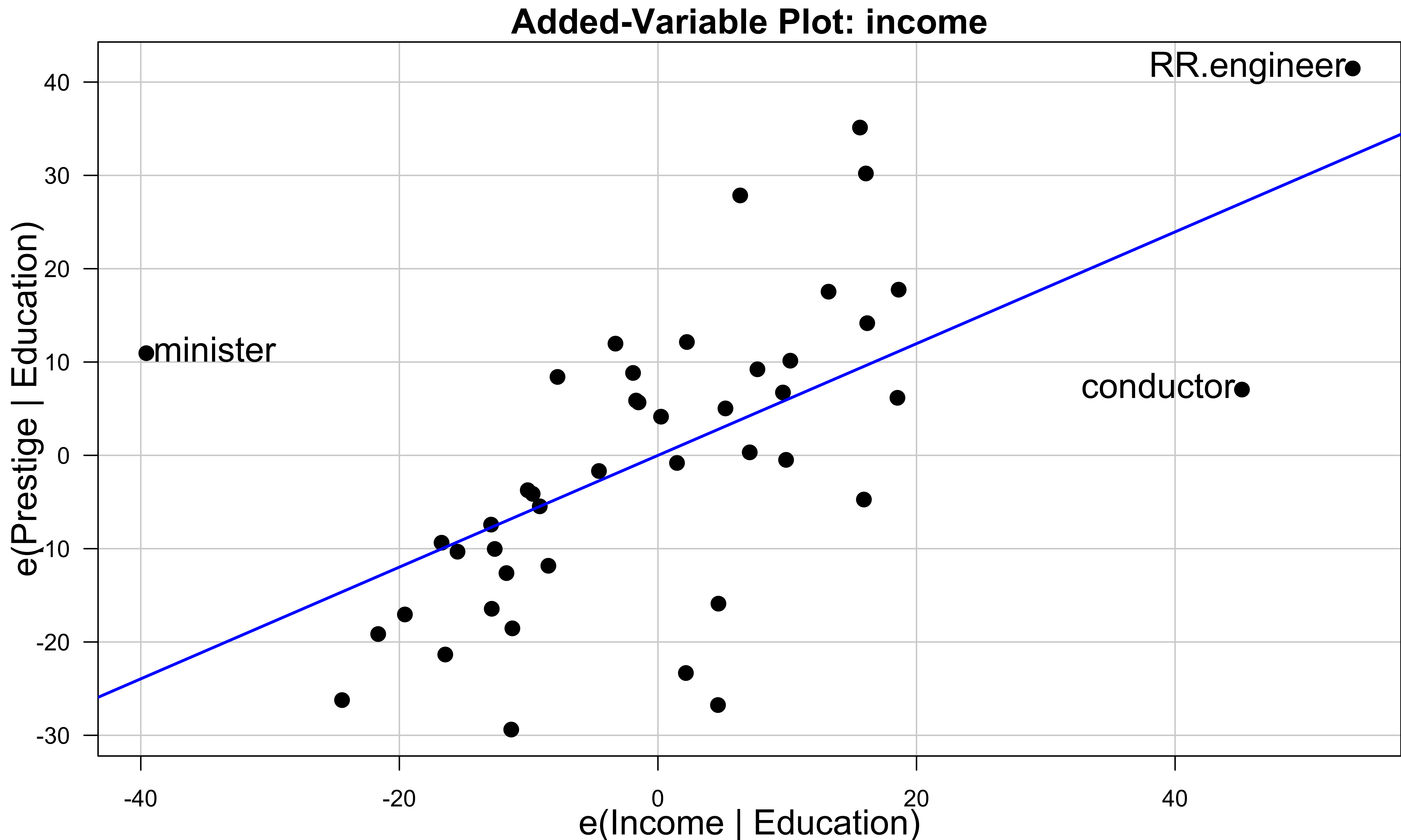
- Minister’s income is low given its education level.
- Railroad engineer and railroad conductor’s income is high given their education level.
- The points for minister and conductor appear to be working jointly to decrease the income slope.
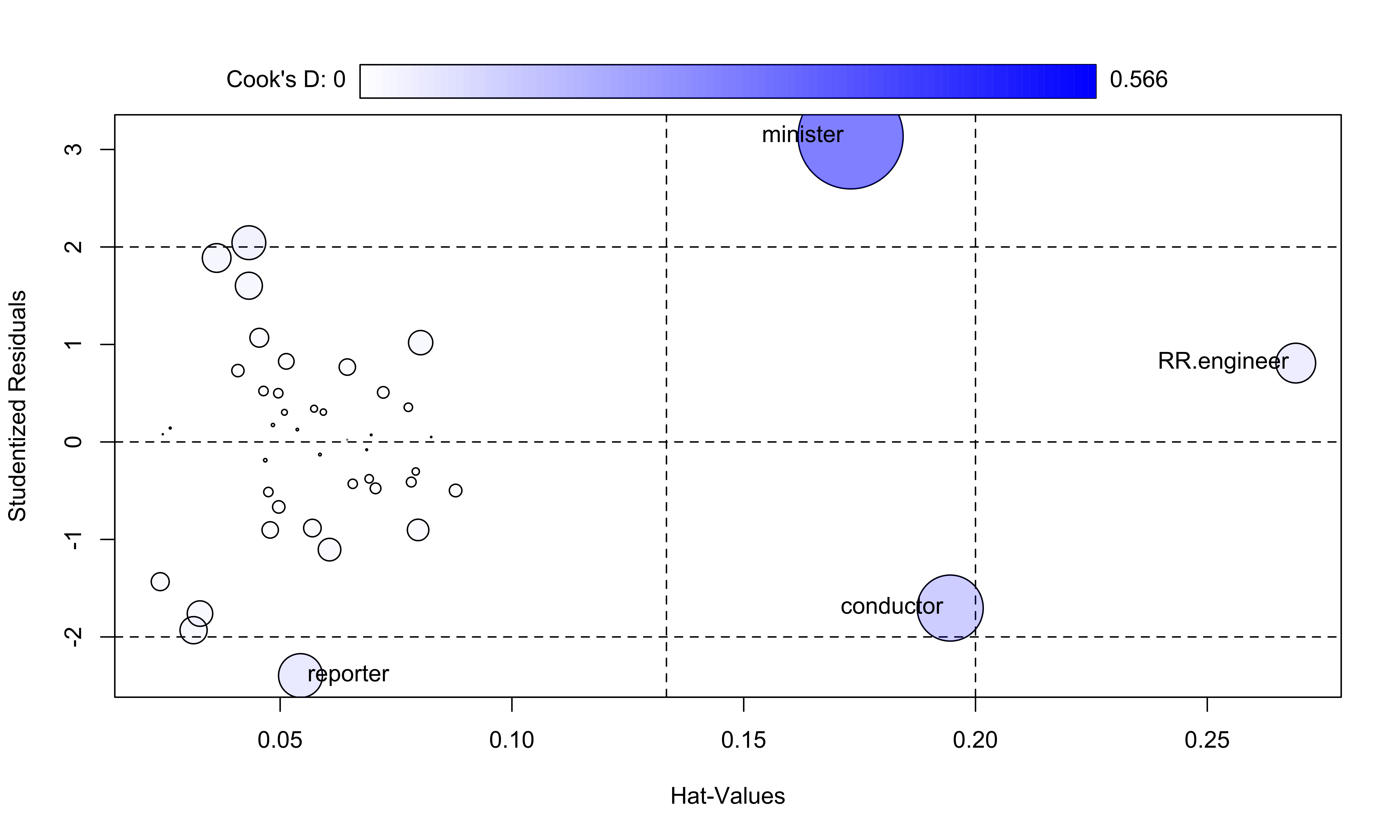
R Lab Bubble Plot
- Each point is plotted as a circle with area proportional to Cook’s distance.
- Horizontal lines are drawn R-Student residuals of 0 and \(\pm 2\).
- The vertical lines at \(2\bar{h}\) and \(3\bar{h}\).
Treatment of Unusual Data
Should unusual data be discarded?
First investigate why data are unusual.
-
Error in recording:
- If the typo can be corrected, correct it and keep it.
- If it cannot be corrected, discard it.
If the unusual point is known to be correct, understand why.
-
Outliers or influential data may also motivate model respecification.
- The pattern of outlying data may suggest introducing additional regressors.
