Multiple Linear Regression 👨‍💻

MATH 4780 / MSSC 5780 Regression Analysis

Dr. Cheng-Han Yu
Department of Mathematical and Statistical Sciences
Marquette University

Multiple Linear Regression Model (MLR)

• All right, we are finally going to talk about MLR. As I mentioned before, MLR is pretty like SLR.
• They share the same idea and concept in terms of prediction and inference.
• The major different is that MLR uses more than one regressor in the model, and we usually use matrix notation to describe a MLR and do calculations.
• It does not mean that we cannot use the math notations used in SLR to express a MLR model. But you’ll find out it is much more tedious if we don’t use matrix, and using matrix algebra makes our life easier.

Why Multiple Regression?

• Our target response may be affected by several factors.
• Total sales \((Y)\) and amount of money spent on advertising on YouTube (YT) \((X_1)\), Facebook (FB) \((X_2)\), Instagram (IG) \((X_3)\).

• Predict sales based on the three advertising expenditures and see which medium is more effective.

• The first question you may ask is Why we want Multiple Regression?
• In practice, we often have more than one predictor.
• How amount of money spent on advertising on different media affect the total sales of some product, we may need more than one predictors.
• Because usually company will spend money on several different media, not just one.
• Data: total sales \((Y)\) and amount of money spent on advertising on TV \((X_1)\), YouTube \((X_2)\), and Instagram \((X_3)\).
• We want to predict sales based on the three advertising expenditures and see which medium is more effective.

Fit Separate Simple Linear Regression Models

Fit three separate independent SLR models:

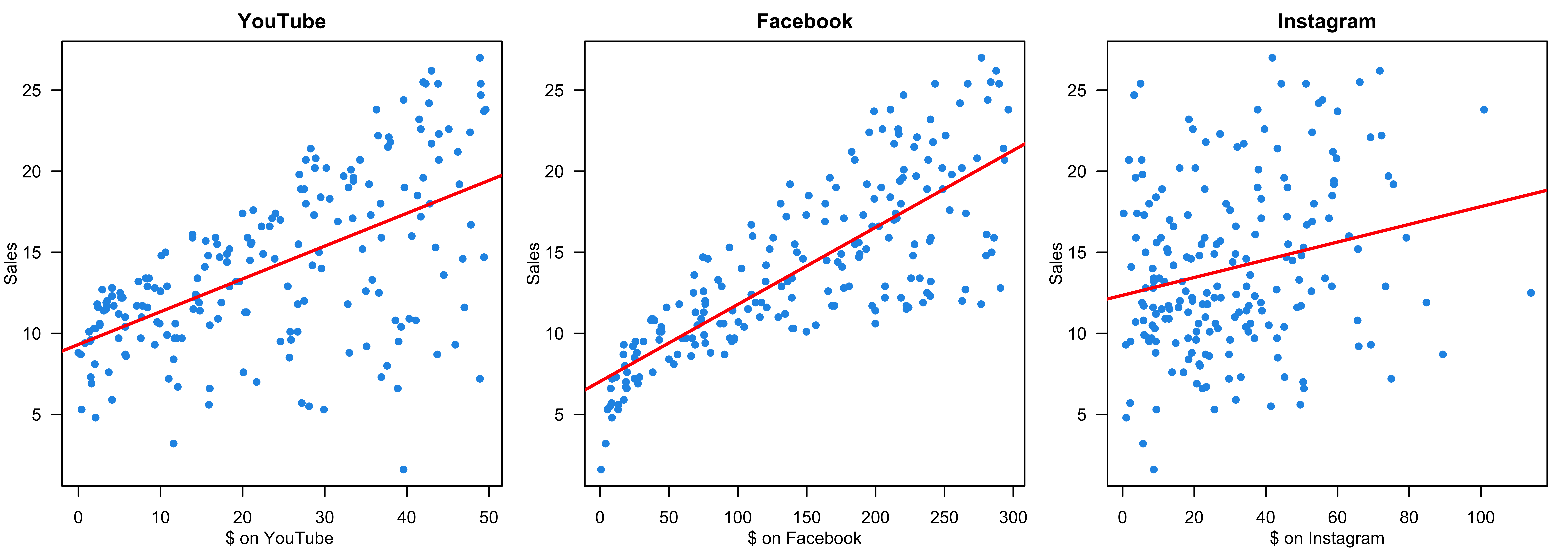
❌ Fitting a separate SLR model for each predictor is not satisfactory.

• You may wonder, how about we just fit three Separate Simple Linear Regression Models, one for each predictor.
• Yes, we could do that. And if we do this, we’ll see that advertising on the 3 media is valuable because the more the money we put in, the higher sales of products we’ll get.
• Fitting a separate SLR model for each predictor is not satisfactory. That’s see why.

Don’t Fit a Separate Simple Linear Regression

• 👉 How to make a single prediction of sales given levels of the 3 advertising media budgets?
  • How to predict the sales when the amount spent on YT is 50, 100 on FB and 30 on IG?

• 👉 Each regression equation ignores the other 2 media in forming coefficient estimates.
  • The effect of FB advertising on sales may be increased or decreased when YT and IG advertising are in the model.
  • IG advertising may have no impact on sales when YT and FB advertising are in the model.

• 👍👍 Better approach: extend the SLR model so that it can directly accommodate multiple predictors.

• Fitting a separate SLR model for each predictor is not satisfactory.
  • It is unclear how to make a single prediction of sales given levels of the three advertising media budgets, since each of the budgets is associated with a separate regression equation.
  • Each of the three regression equations ignores the other two media in forming estimates for the regression coefficients.
  • If the three media budgets are correlated with each other, this can lead to very misleading estimates of the individual media effects on sales.
• A better approach is to extend the simple linear regression model so that it can directly accommodate multiple predictors.

I hope you don’t feel…

Source: https://memegenerator.net/instance/62248186/first-world-problems-multiple-regression-more-like-multiple-depression

What I hope is…

https://www.tldrpharmacy.com/content/how-to-be-awesome-at-biostatistics-and-literature-evaluation-part-iii

Multiple Linear Regression (MLR) Model

• We have \(k\) distinct predictors. The (population) multiple linear regression model: \[Y_i= \beta_0 + \beta_1X_{i1} + \beta_2X_{i2} + \dots + \beta_kX_{ik} + \epsilon_i\]
• \(X_{ij}\): \(j\)-th regressor value on \(i\)-th measurement, \(j = 1, \dots, k\).
• \(\beta_j\): \(j\)-th coefficient quantifying the association between \(X_j\) and \(Y\).

• In the advertising example, \(k = 3\) and \[\texttt{sales} = \beta_0 + \beta_1 \times \texttt{YouTube} + \beta_2 \times \texttt{Facebook} + \beta_3 \times \texttt{Instagram} + \epsilon\]

• Assumptions as SLR
  • \(\epsilon_i \stackrel{iid}{\sim} N(0, \sigma^2)\)

• When \(k = 1\), MLR is reduced to SLR.

• Two subscripts of X.
• Later, we will learn how to interpret the coefficients correctly.
• We interpret \(\beta_j\), \(j = 1, \dots, p\), as the average effect on \(Y\) of a one unit increase in \(X_j\), holding all other predictors fixed.

How many parameters are there in the model?

Sample MLR Model

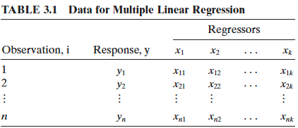
• Given the training sample data \((x_{11}, \dots, x_{1k}, y_1), (x_{21}, \dots, x_{2k}, y_2), \dots, (x_{n1}, \dots, x_{nk}, y_n),\)
• The sample MLR model: \[\begin{align} y_i &= \beta_0 + \beta_1x_{i1} + \beta_2x_{i2} + \dots + \beta_k x_{ik} + \epsilon_i \\ &= \beta_0 + \sum_{j=1}^k\beta_j x_{ij} + \epsilon_i, \quad i = 1, 2, \dots, n \end{align}\]

• Writing our data and model without using matrix starts getting tedious.
• Later we’ll see our to write it in a more clean way using matrix notation.
• our mpg data set in the homework has this type of structure.
• In R we usually store this kind of data set in R structure call data frame.

Regression Hyperplane

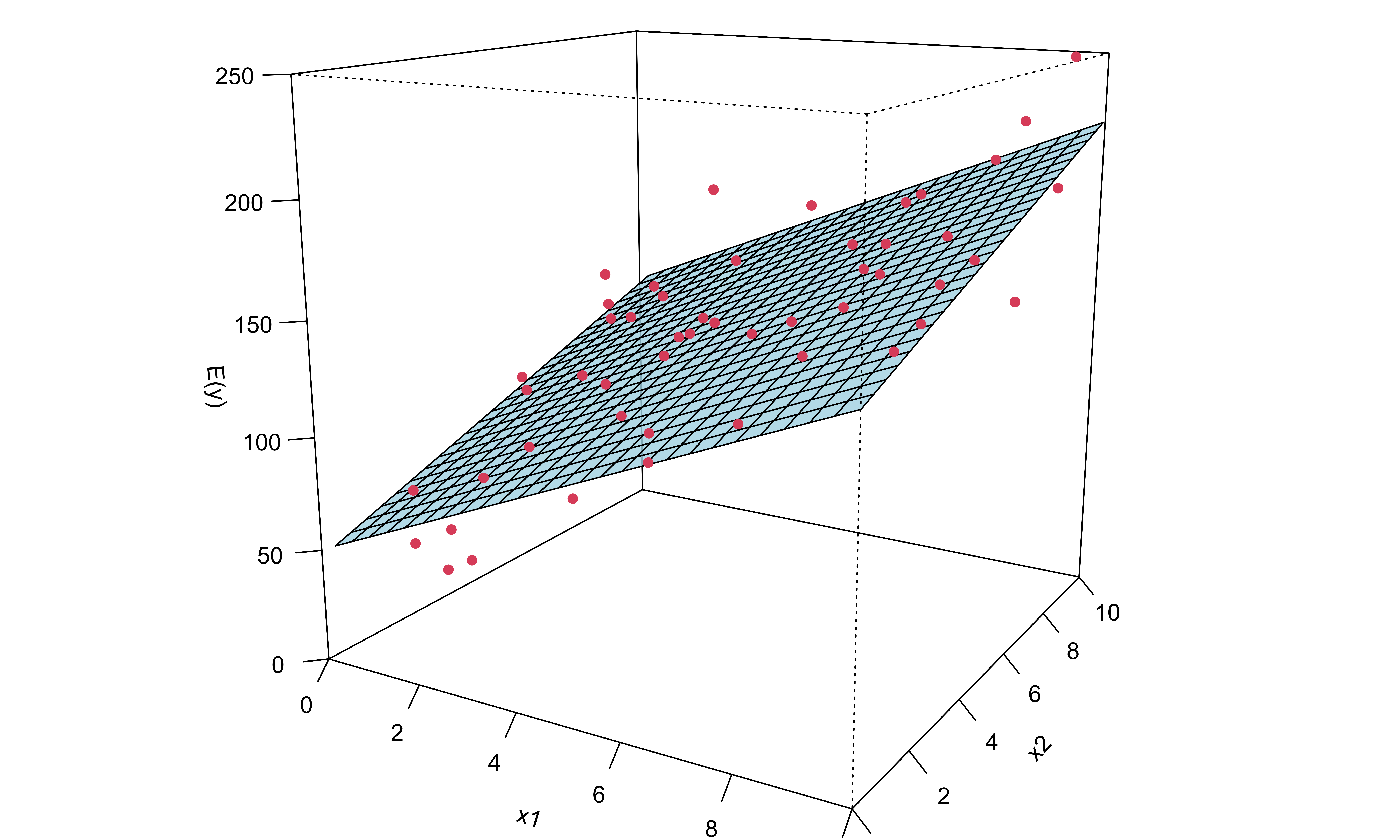
• SLR: regression line
• MLR: regression hyperplane or response surface
• \(y = \beta_0 + \beta_1x_1 + \beta_{2}x_2 + \epsilon\)
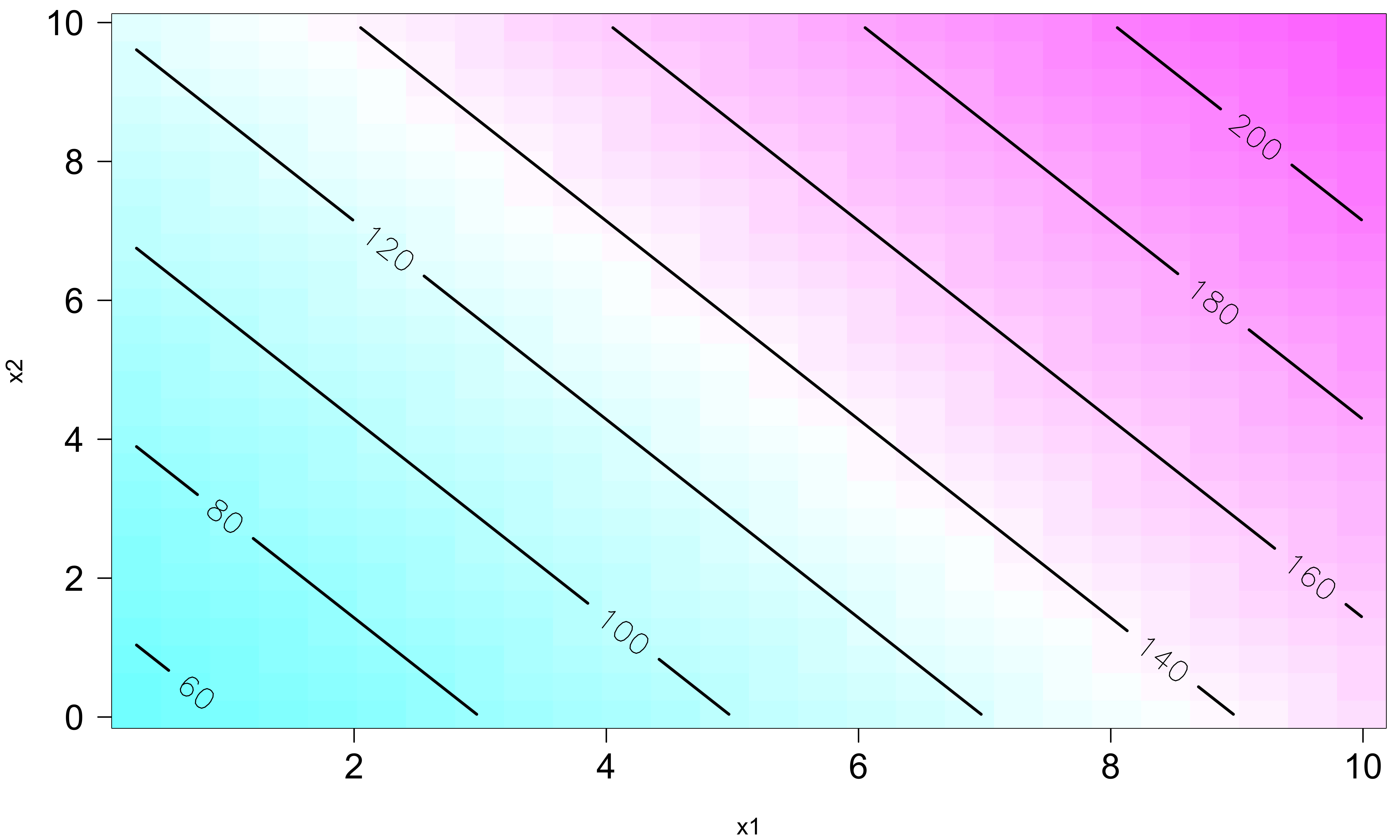
• \(E(y \mid x_1, x_2) = 50 + 10x_1 + 7x_2\)

• Now I’m gonna show you what a MLR looks like when we fit it to the data.

• If we have two predictors, we will have a sample regression plane.

• If we have more than two predictors in the model, we are not able to visualize it, but the idea is the same.

• We will have a something called hyperplane or response surface that basically play the same role as the regression plane in 2D or regression line in 1D.

• The plot on the right is the contour plot when we project the plot onto the x1-x2 plane. You can see that basically the higher x1 and/or the higher x2, the higher value of y.

• Moreover, you can see that the level curves are straight and parallel, meaning that the effect of x1 on y does not change with the values of x2 or the effect does not depend on the level of x2.

• https://cran.r-project.org/web/packages/rsm/vignettes/rsm-plots.pdf

• http://www.sthda.com/english/wiki/scatterplot3d-3d-graphics-r-software-and-data-visualization

• https://stackoverflow.com/questions/18147595/plot-3d-plane-true-regression-surface

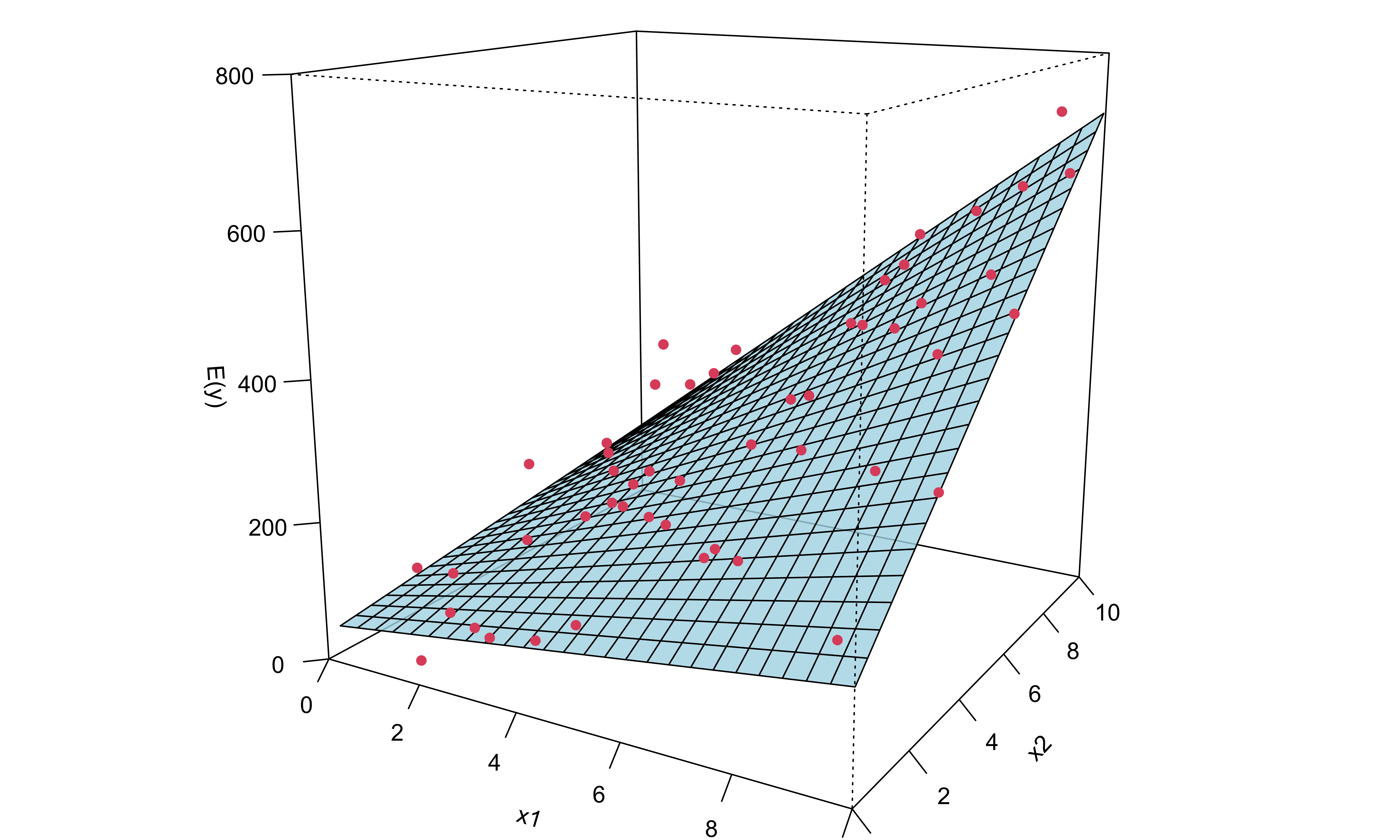
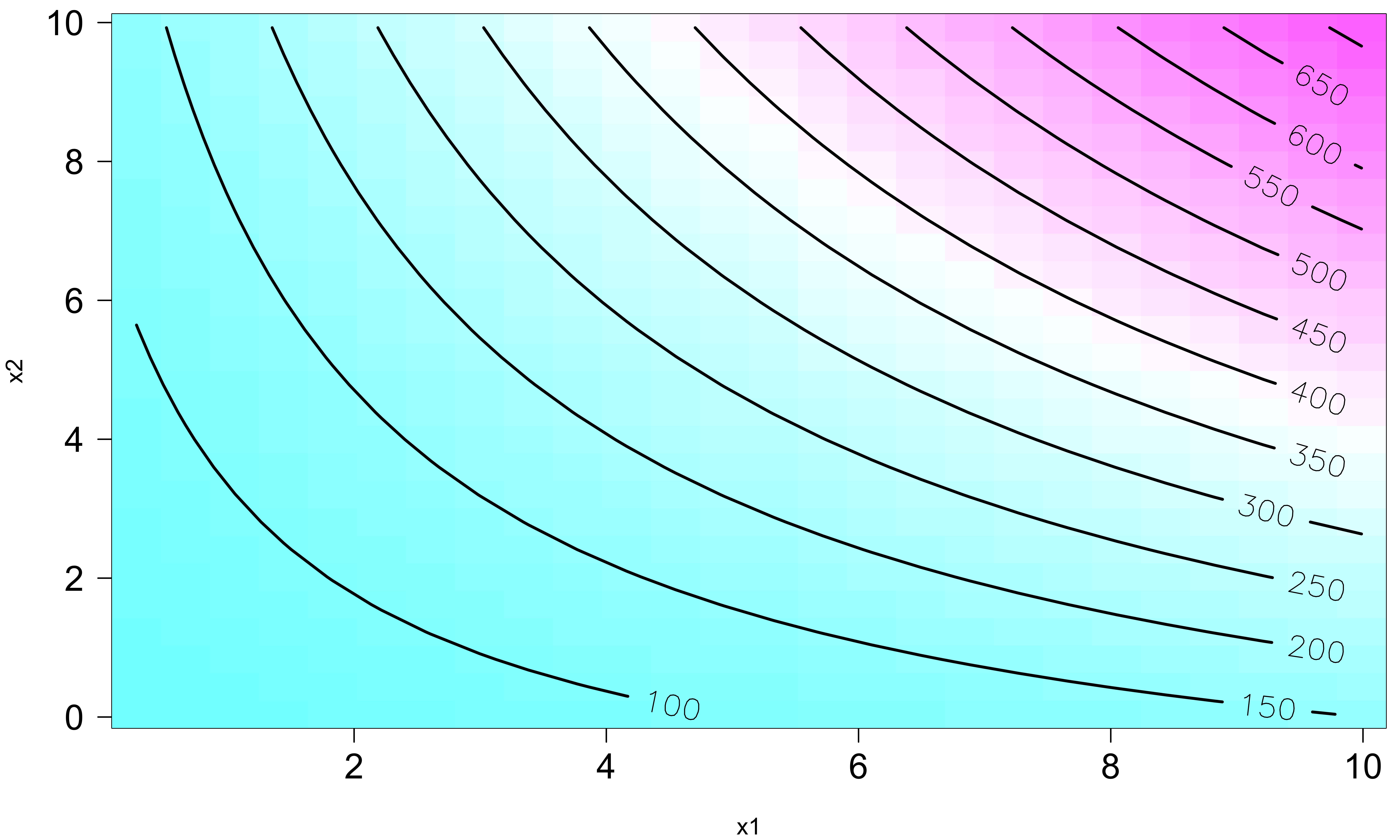
Response Surface : Interaction Model

• \(y = \beta_0 + \beta_1x_1 + \beta_{2}x_2 + \beta_{12}x_1x_2 + \epsilon\)
• This is in fact a linear regression model: let \(\beta_3 = \beta_{12}, x_3 = x_1x_2\).
• \(E(y \mid x_1, x_2) = 50 + 10x_1 + 7x_2 + 5x_1x_2\)
• 😎 🤓 A linear model generates a nonlinear response surface!

• Remember in SLR, we can have a liner model that describes a nonlinear relationship.
• Same in MLR. We can have a linear model that generates a nonlinear response surface!
• \(y = \beta_0 + \beta_1x_1 + \beta_{2}x_2 + \beta_{12}x_1x_2 + \epsilon\)
• This is in fact a linear regression model: let \(\beta_3 = \beta_{12}, x_3 = x_1x_2\).

Response Surface : 2nd Order with Interaction Model

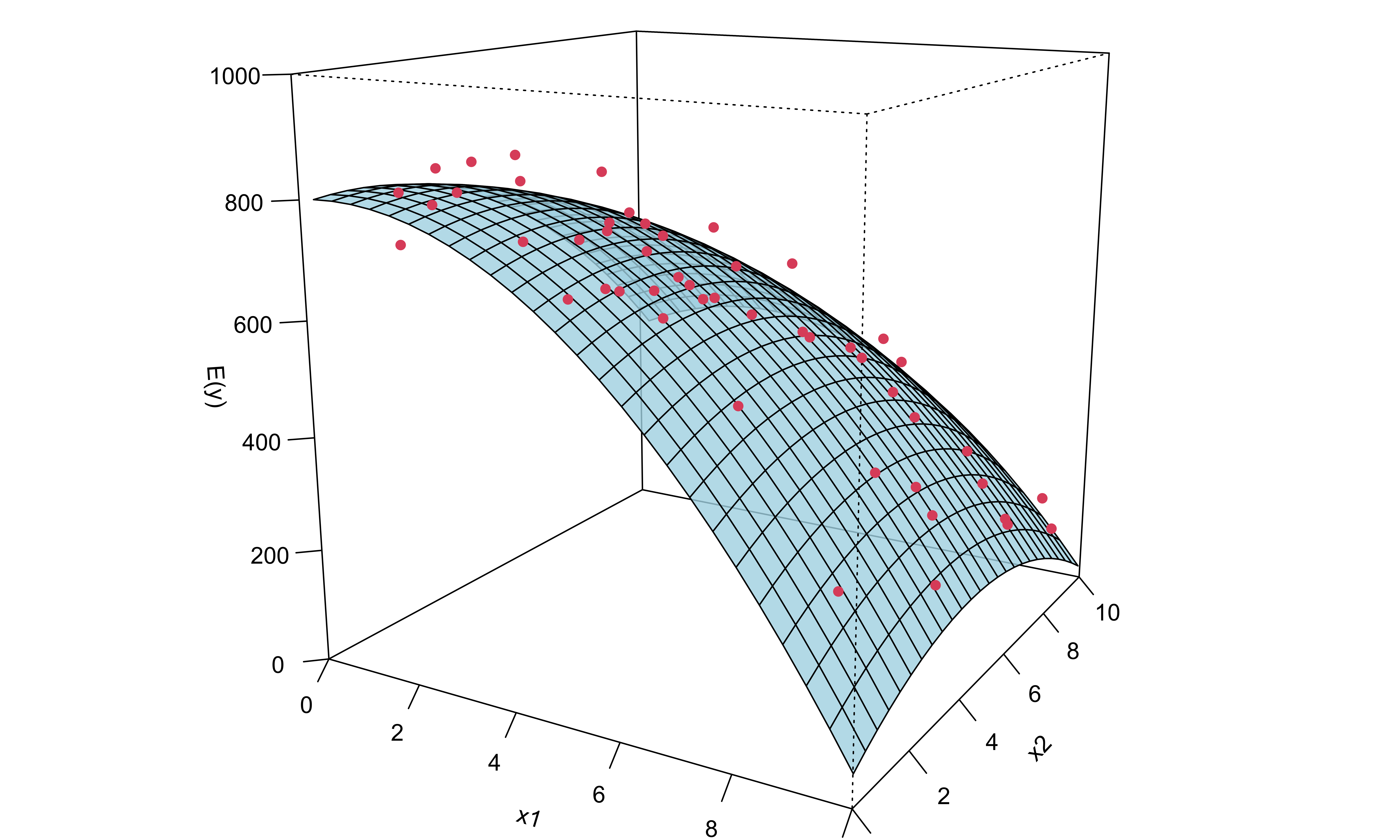
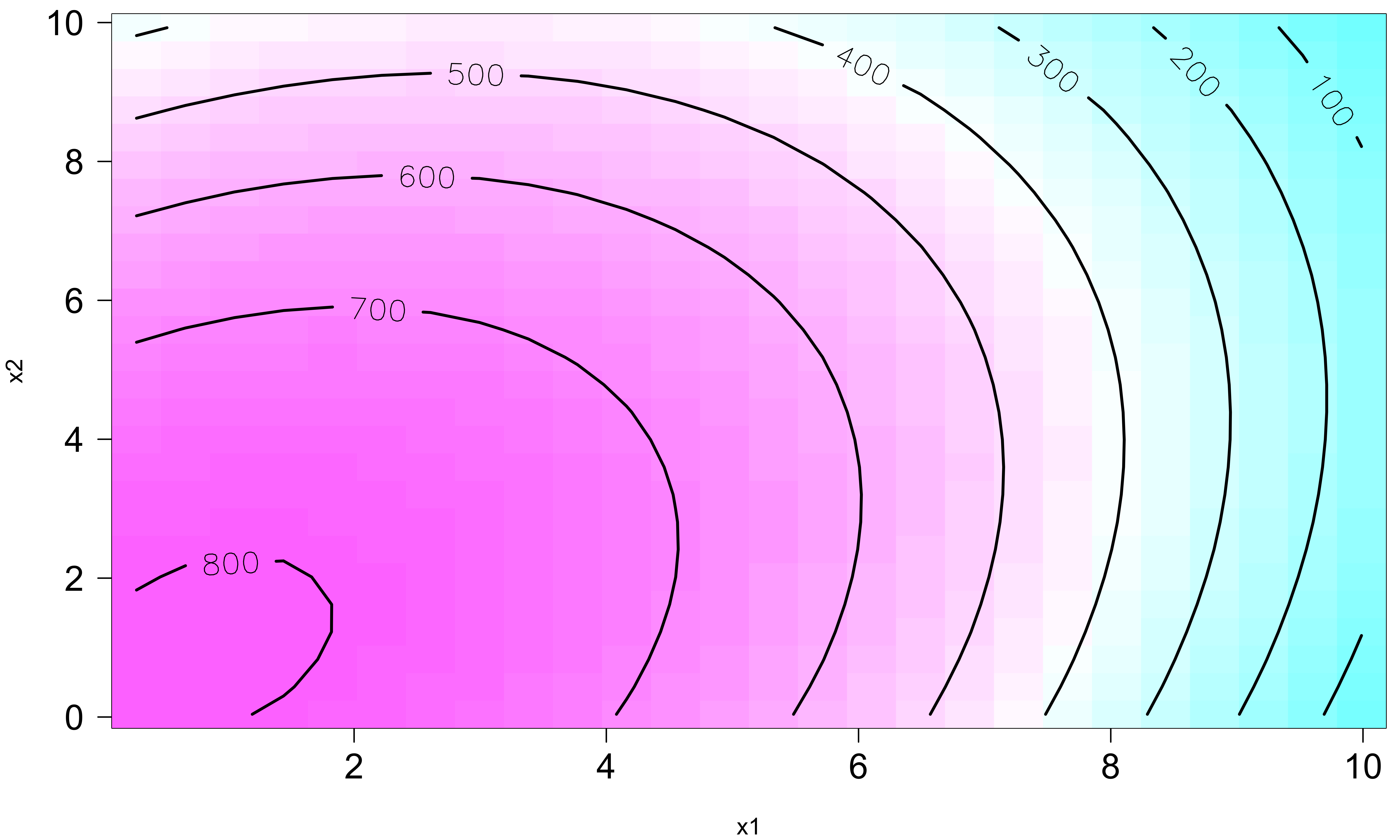
• \(y = \beta_0 + \beta_1x_1 + \beta_{2}x_2 + \beta_{11}x_1^2 + \beta_{22}x_2^2 + \beta_{12}x_1x_2 + \epsilon\)
• \(E(y) = 800+10x_1+7x_2 -8.5x_1^2-5x_2^2- 4x_1x_2\)
• 😎 🤓 A linear regression model can describe a complex nonlinear relationship between the response and predictors!

Point Estimation of Model Parameters

Least Square Estimation of the Coefficients

\[\begin{align} y_i &= \beta_0 + \beta_1x_{i1} + \beta_2x_{i2} + \dots + \beta_k x_{ik} + \epsilon_i \\ &= \beta_0 + \sum_{j=1}^k\beta_j x_{ij} + \epsilon_i, \quad i = 1, 2, \dots, n \end{align}\]

• The least-squares function is \[S(\alpha_0, \alpha_1, \dots, \alpha_k) = \sum_{i=1}^n\left(y_i - \alpha_0 - \sum_{j=1}^k\alpha_j x_{ij}\right)^2\] The function \(S(\cdot)\) must be minimized with respect to the coefficients, i.e., \[(b_0, b_1, \dots, b_k) = \underset{{\alpha_0, \alpha_1, \dots, \alpha_k}}{\mathrm{arg \, min}} S(\alpha_0, \alpha_1, \dots, \alpha_k)\]

• As SLR, we can define the least-squares function as the sum of squares of epsilon.
• The idea is to minimize the function \(S\) w.r.t. the model coefficients \(\beta_0, \beta_1, \dots, \beta_k\).
• In other words, we are going to choose the sample statistics \(b_0\), \(b_1\), …, \(b_k\) as the estimates of \(\beta_0, \beta_1, \dots, \beta_k\) so that \(S(.)\) is minimized when \(b_0\), \(b_1\), …, \(b_k\) are plugged in the function.

Geometry of Least Square Estimation

• If we look at the geometry of Least Square Estimation of the MLR, we have a visualization like this.
• Again, in SLR, different \(b_0\) and \(b_1\)s give us different sample regression lines.
• In MLR, suppose we have two predictors, and different \(b_0\) and \(b_1\) and \(b_2\) give us different sample regression planes.
• so geometrically speaking, we are trying to find a sample regression plane such that the sum of the squared distance between the observations (denoted by those blue points) and the plane is minimized.
• For more than 2 predictor case, we are not able to visualize it because we live a 3D world, but the idea is exactly the same. And we called the regression plane a hyperplane. OK.

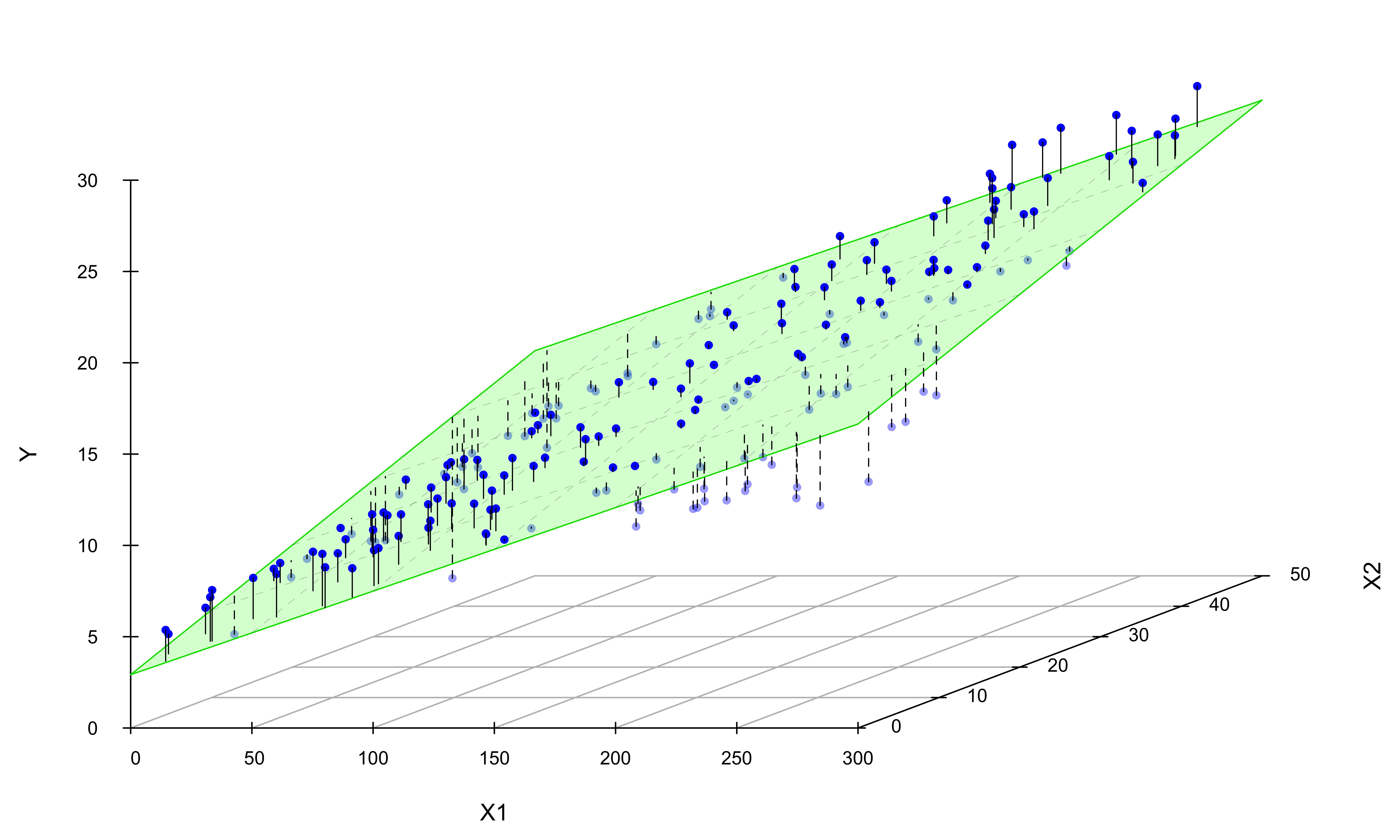
Least-squares Normal Equations

\[\begin{align} \left.\frac{\partial S}{\partial\alpha_0}\right\vert_{b_0, b_1, \dots, b_k} &= -2 \sum_{i=1}^n\left(y_i - b_0 - \sum_{j=1}^k b_j x_{ij}\right) = 0\\ \left.\frac{\partial S}{\partial\alpha_j}\right\vert_{b_0, b_1, \dots, b_k} &= -2 \sum_{i=1}^n\left(y_i - b_0 - \sum_{j=1}^k b_j x_{ij}\right)x_{ij} = 0, \quad j = 1, 2, \dots, k \end{align}\]

• \(p = k + 1\) equations with \(p\) unknown parameters.
• The ordinary least squares estimators are the solutions to the normal equations.

• So again similar to SLR, we can take derivative w.r.t \(\beta_0\), \(\beta_1\), to the \(\beta_k\).
• And we are gonna have \(p = k + 1\) equations with \(p\) unknown parameters.
• So we can find one and only one solution to \(\beta_0\), \(\beta_1\), to the \(\beta_k\), which are \(b_0\), \(b_1\), …, \(b_k\).
• And the \(p\) equations are the least squares normal questions.
• You guys solve the equations when k = 1.
• Do you think it is easy to solve the questions when the number of predictors is 2 or more than 2?

🍹 🍺 🍸 🥂 I buy you a drink if you solve the equations for \(k \ge 2\) by hand without using matrix notations or operations!

• Here I am happy to treat you and buy you a drink if you can solve the equations for \(k \ge 2\) by hand without using matrix notations or operations!
• Come to my office hours and show your work. And we go to a bar together. Sounds good?
• In fact, if you try, you are gonna deal with lots of algebra, but if we write the system of equations in a matrix form, the solution becomes very clean.
• That’s see why.

R Lab Delivery Time Data

# Load the data set
delivery <- read.csv(file = "./data/data-ex-3-1.csv",
                     header = TRUE)
delivery_data <- delivery[, -1]
colnames(delivery_data) <- c("time", "cases", "distance")
str(delivery_data)

'data.frame':   25 obs. of  3 variables:
 $ time    : num  16.7 11.5 12 14.9 13.8 ...
 $ cases   : int  7 3 3 4 6 7 2 7 30 5 ...
 $ distance: int  560 220 340 80 150 330 110 210 1460 605 ...

• \(y\): the amount of time required by the route driver to stock the vending machines with beverages
• \(x_1\): the number of cases stocked
• \(x_2\): the distance walked by the driver

delivery_data

   time cases distance
1  16.7     7      560
2  11.5     3      220
3  12.0     3      340
4  14.9     4       80
5  13.8     6      150
6  18.1     7      330
7   8.0     2      110
8  17.8     7      210
9  79.2    30     1460
10 21.5     5      605
11 40.3    16      688
12 21.0    10      215
13 13.5     4      255
14 19.8     6      462
15 24.0     9      448
16 29.0    10      776
17 15.3     6      200
18 19.0     7      132
19  9.5     3       36
20 35.1    17      770
21 17.9    10      140
22 52.3    26      810
23 18.8     9      450
24 19.8     8      635
25 10.8     4      150

• \(y\): the amount of time required by the route driver to stock the vending machines with beverages in an outlet.
• \(x_1\): the number of cases stocked
• \(x_2\): the distance walked by the driver
• Goal: fit a MLR model \(y = \beta_0 + \beta_1x_1 + \beta_2x_2 + \epsilon\) to the amount of time required by the route driver to service the vending machines (use readr::read_csv if the file is large)

R Lab Scatterplot Matrix

pairs(delivery_data)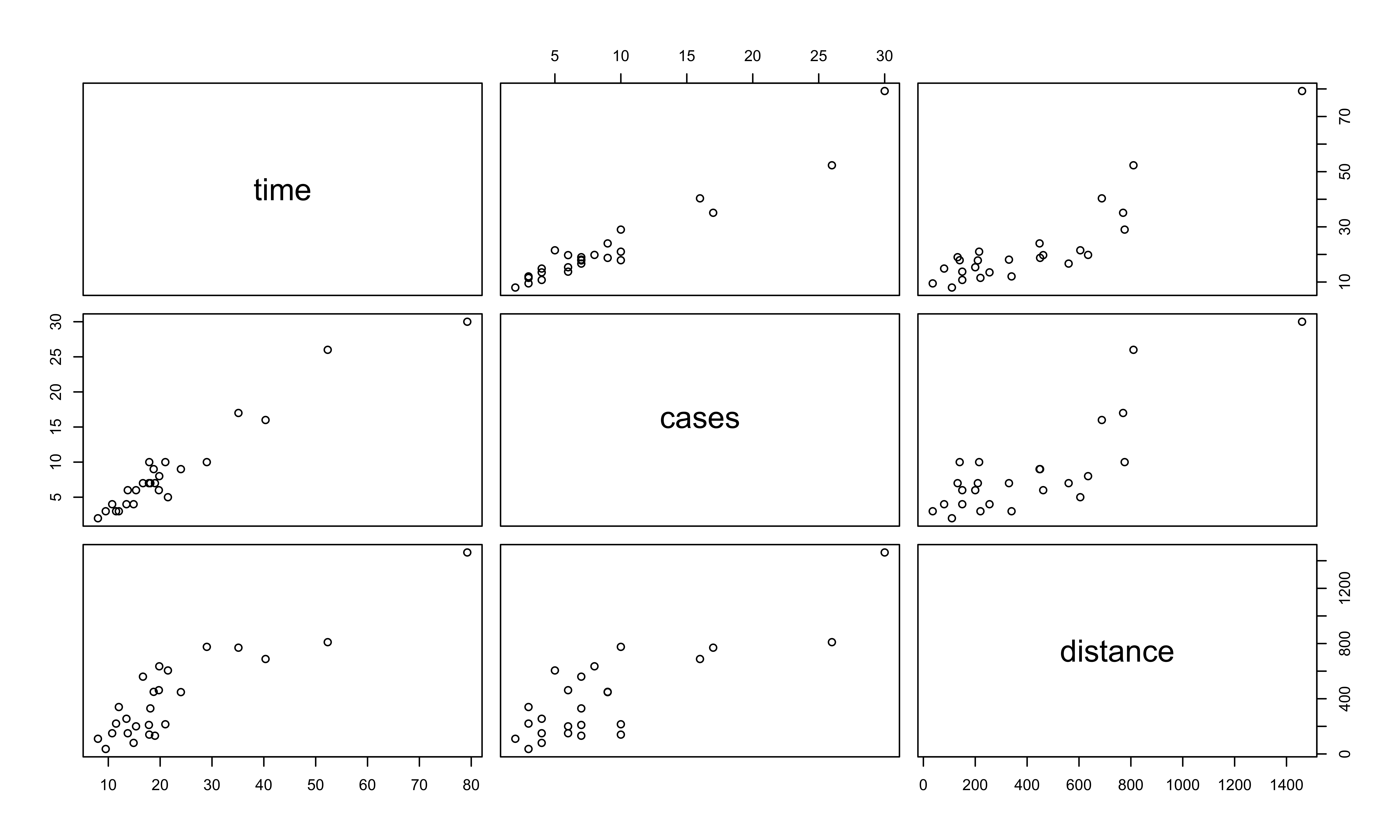

• Each plot shows the relationship between a pair of variables.

R Lab 3D Scatterplot

Code

par(mgp = c(2, 0.8, 0), las = 1, mar = c(4, 4, 0, 0))
library(scatterplot3d)
scatterplot3d(x = delivery_data$cases, y = delivery_data$distance, z = delivery_data$time,
              xlab ="cases", ylab = "distance", zlab = "time",
              xlim = c(2, 30), ylim = c(36, 1640), zlim = c(8, 80),
              box = TRUE, color = "blue", mar = c(3, 3, 0, 2), angle = 30, pch = 16)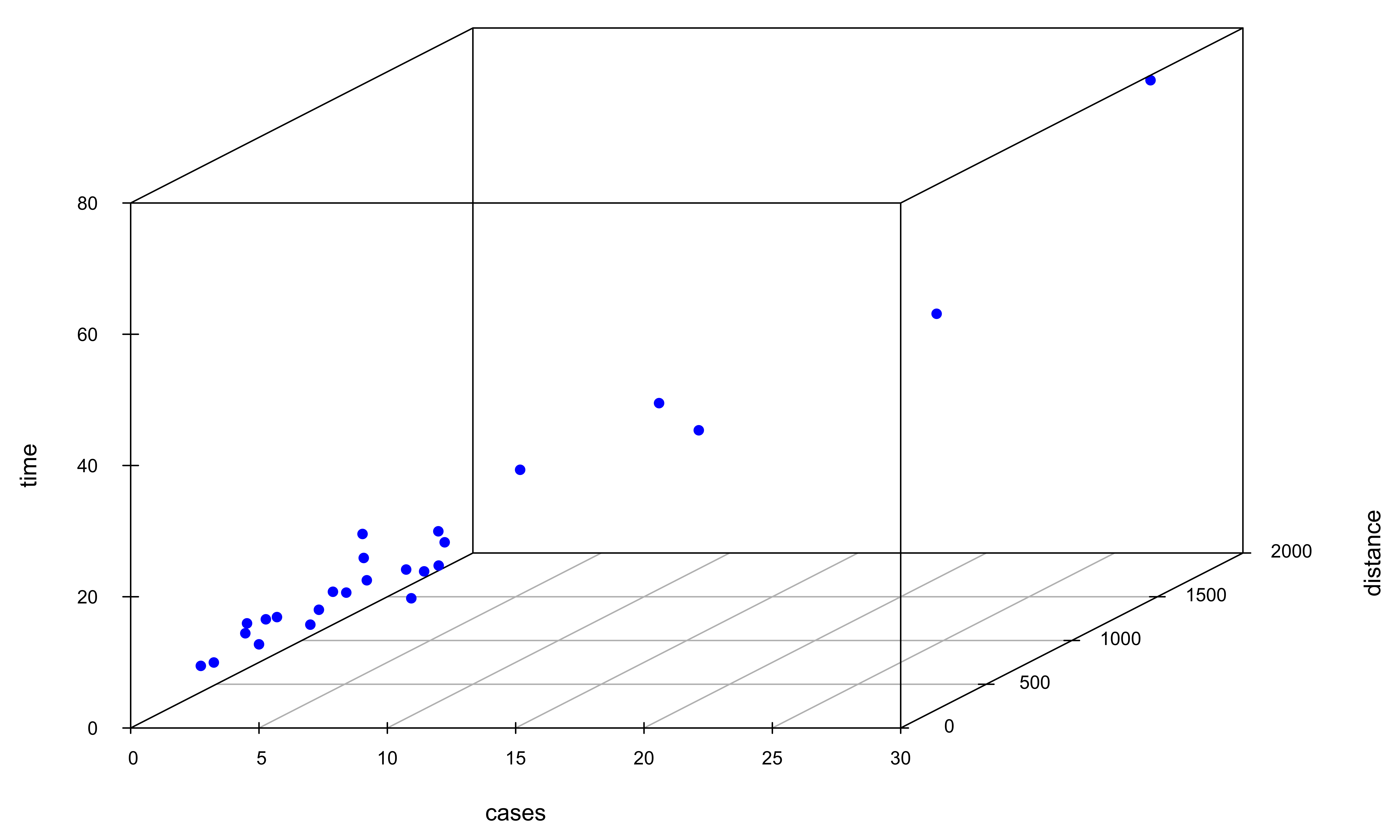

• Sometimes a 3D scatterplot is useful in visualizing the relationship between the response and the regressors when there are only two regressors.

R Lab Multiple Linear Regression

delivery_lm <- lm(time ~ cases + distance, data = delivery_data)
delivery_lm$coef

(Intercept)       cases    distance 
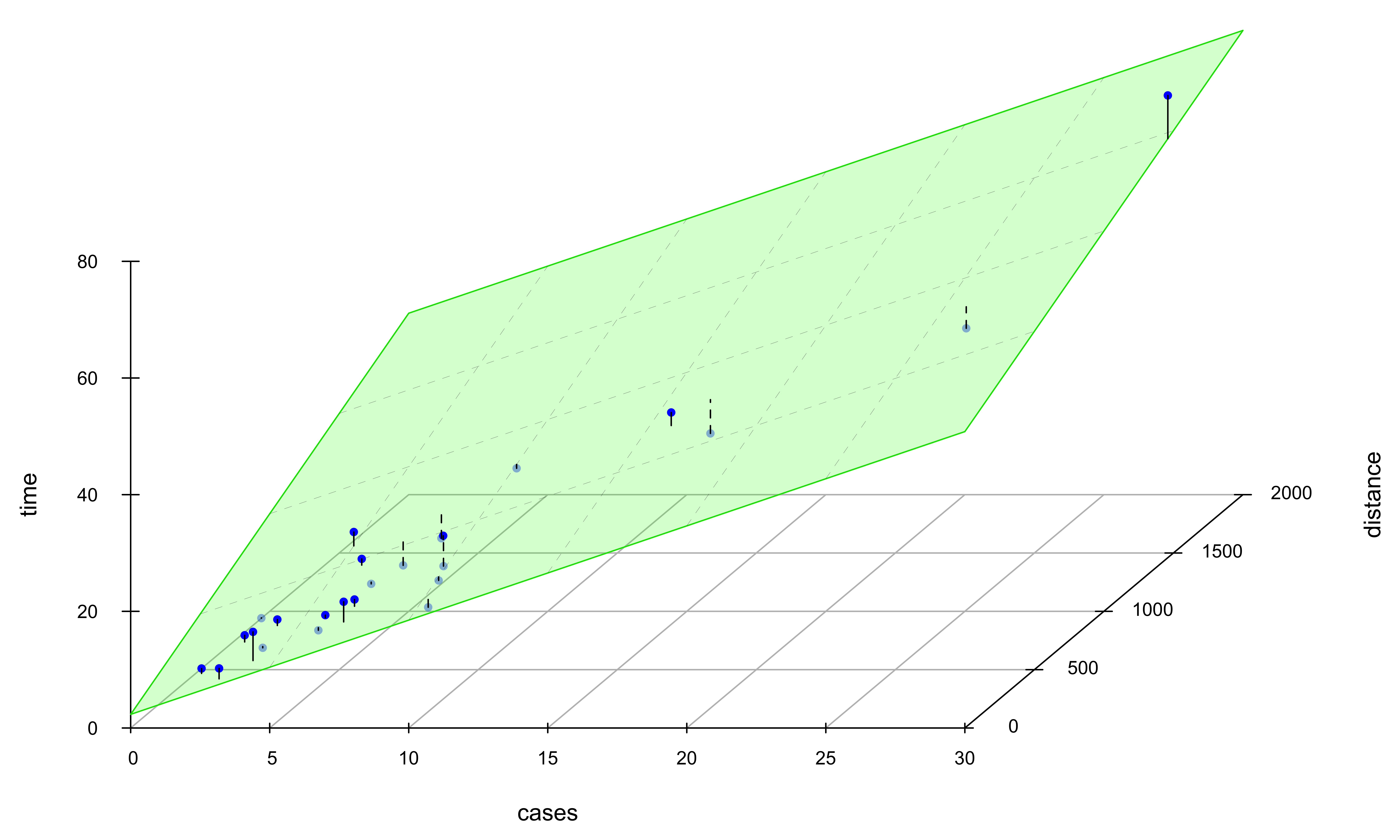
      2.341       1.616       0.014 

\[\hat{y} = 2.34 + 1.62x_1 + 0.014x_2\]

• \(b_1\): All else held constant, for one case of product stocked increase, we expect the delivery time to be longer, on average, by 1.62 minutes.

• \(b_2\): All else held constant, one additional foot walked by the driver causes the delivery time, on average, to be 0.014 minutes longer.

• \(b_0\): The delivery time with no number of cases of product stocked and no distance walked by the driver is expected to be 2.34 minutes. (Make sense?!)

R Lab Regression Plane

Estimation of \(\sigma^2\)

• \(SS_{res} = \sum_{i=1}^ne_i^2 = \sum_{i=1}^n(y_i - \hat{y}_i)^2\).

• \(MS_{res} = \frac{SS_{res}}{n - p}\) with \(p = k + 1\).

• \(S^2 = MS_{res}\) is unbiased for \(\sigma^2\), i.e., \(E[MS_{res}] = \sigma^2\).

• \(S^2\) of SLR may be quite larger than the \(S^2\) of MLR.

• \(S^2\) measures the variation of the unexplained noise about the fitted regression line/hyperplane, so we prefer a small residual mean square.

• \(SS_{res} = \sum_{i=1}^ne_i^2 = {\bf e'e} = {\bf (y-Xb)'(y-Xb)} = {\bf y'y - b'X'y} = \sum_{i=1}^n(y_i - \hat{y}_i)^2\).
• If our model is specified correctly, \(\hat{\sigma}^2\) depends on our data quality.
• If our data have lots of noise itself, there is nothing we can do.

R Lab Estimation of \(\sigma^2\)

## method 1
summ_delivery <- summary(delivery_lm)  ## check names(summ_delivery)
summ_delivery$sigma ^ 2

[1] 11

## method 2
n <- length(delivery_lm$residuals)
(SS_res <- sum(delivery_lm$residuals * delivery_lm$residuals))

[1] 234

SS_res / (n - 3)

[1] 11

## method 3
(SS_res1 <- sum((delivery_data$time - delivery_lm$fitted.values) ^ 2))

[1] 234

SS_res1 / (n - 3)

[1] 11

Confidence Interval

CI for Coefficients

CI for the Mean Response

PI for New Observations

Properties of LSEs

• 👍 \({\bf b} = (b_0, b_1, \dots, b_k)'\) is BLUE.
• Linear : Each \(b_j\) is a linear combination of \(y_1, \dots, y_n\).
• Unbiased : Each \(b_j\) is normally distributed with mean \(\beta_j\).
• Best : Each \(b_j\) has the minimum variance, comparing to all other unbiased estimator for \(\beta_j\) that is a linear combo of \(y_1, \dots, y_n\).

Wald CI for Coefficients

The \((1-\alpha)100\%\) Wald CI for \(\beta_j\), \(j = 0, 1, \dots, k\) is \[\left(b_j- t_{\alpha/2, n-p}~se(b_j), \quad b_j + t_{\alpha/2, n-p}~ se(b_j)\right)\]

(ci <- confint(delivery_lm))

             2.5 % 97.5 %
(Intercept) 0.0668  4.616
cases       1.2618  1.970
distance    0.0069  0.022

• These are marginal CIs seperately for each \(b_j\).

• Each of the statistics \(\frac{b_j - \beta_j}{\sqrt{\hat{\sigma}^2C_{jj}}}, j = 0, 1, 2, \dots, k\) follows \(t_{n-p}\) distribution, where \(\hat{\sigma}^2 = MS_{res}\), and \(C_{jj}\) is the \(j\)-th diagonal element of \({\bf (X'X)}^{-1}\).
• The \((1-\alpha)100\%\) CI for \(\beta_j\), \(j = 0, 1, \dots, k\) is \(\left(b_j- t_{\alpha/2, n-p} \sqrt{\hat{\sigma}^2C_{jj}}, \quad b_j + t_{\alpha/2, n-p} \sqrt{\hat{\sigma}^2C_{jj}}\right)\)
• These interval estimates do not take correlation of coefficients into account. One coefficient may be higher when another is lower.
• We can only use the intervals one at a time when doing interval estimation. When we want to do interval estimation for several coefficients together at the same time, these intervals are not that accurate.

Correlated Coefficients

## variance-covariance matrix
V <- vcov(delivery_lm)

## standard error
sqrt(diag(V))

(Intercept)       cases    distance 
     1.0967      0.1707      0.0036 

## correlation matrix
cov2cor(V)

            (Intercept) cases distance
(Intercept)        1.00 -0.25    -0.22
cases             -0.25  1.00    -0.82
distance          -0.22 -0.82     1.00

• \(b_1\) and \(b_2\) are negatively correlated.

• Individual CI ignores the correlation between \(b_j\)s.

How do we specify a confidence level that applies simultaneously to a set of interval estimates? For example, a \(95\%\) confidence “interval” for both \(b_1\) and \(b_2\).

Confidence Region

• The \((1-\alpha)100\%\) CI for a set of \(b_j\)s will be an elliptically-shaped region!

Code

par(mgp = c(2.8, 0.9, 0), mar = c(4, 4, 2, 0))
## confidence region
car::confidenceEllipse(
    delivery_lm, 
    levels = 0.95, 
    which.coef = c("cases", "distance"), 
    main = expression(
        paste("95% Confidence Region for ", 
              beta[1], " and ",  beta[2])
        )
    )
## marginal CI for cases
abline(v = ci[2, ], lty = 2, lwd = 2)  
## marginal CI for distance
abline(h = ci[3, ], lty = 2, lwd = 2)
points(x = 1.4, y = 0.01, col = "red", cex = 2, pch = 16)
points(x = 2, y = 0.008, col = "black", cex = 2, pch = 16)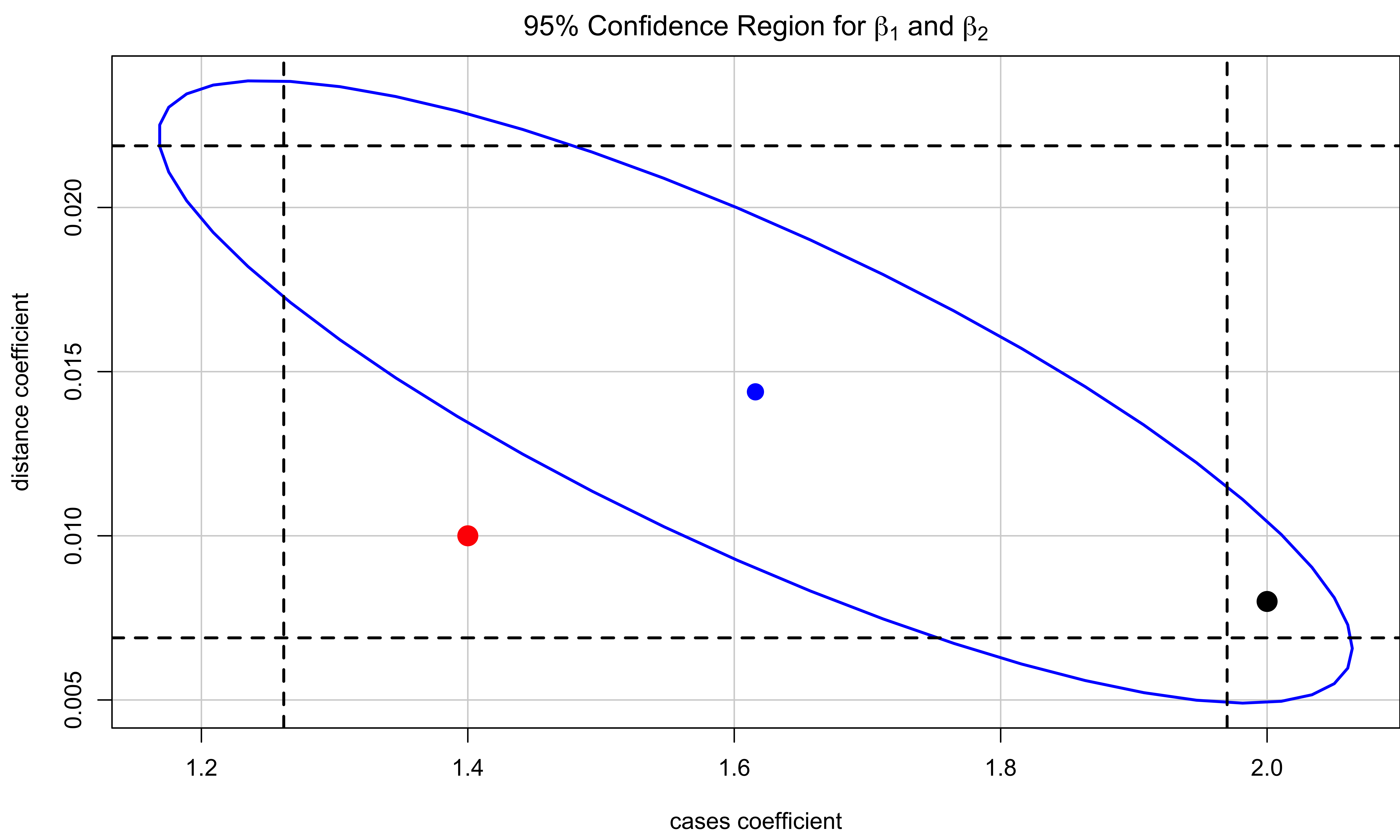

• Some points (red) within the marginal intervals are implausible according to the joint region.
• The joint region includes values of the coefficient for cases (black), for example, that are excluded from the marginal interval.

• Bonferroni
• Scheffe S-method
• maximum modulus t procedure With repeated sampling, 95% of such ellipses will simultaneously include β1 and β2, if the fitted model is correct and normality holds. The orientation of the ellipse reflects the negative correlation between the estimates. Contrast the 95% confidence ellipse with the marginal 95% confidence intervals, also shown on the plot. Some points within the marginal intervals—with larger values for both of the coefficients, for example—are implausible according to the joint region. Similarly, the joint region includes values of the coefficient for income, for example, that are excluded from the marginal interval.

CI for the Mean Response \(E(y \mid {\bf x}_0)\)

• The fitted value at a point \({\bf x}_0 = (1, x_{01}, x_{02}, \dots, x_{0k})'\) is \[\hat{y}_0 = b_0 + b_1x_{01} + \cdots + b_kx_{0k}\]
• This is an unbiased estimator for \(E(y \mid {\bf x}_0)\)
• The \((1-\alpha)100\%\) CI for \(E(y \mid {\bf x}_0)\) is \[\left(\hat{y}_0 - t_{\alpha/2, n-p} ~ se(\hat{y}_0), \quad \hat{y}_0 + t_{\alpha/2, n-p} ~ se(\hat{y}_0)\right)\]

predict(delivery_lm,
        newdata = data.frame(cases = 8, distance = 275),
        interval = "confidence", level = 0.95)

  fit lwr upr
1  19  18  21

• The fitted value at a point \({\bf x}_0 = (1, x_{01}, x_{02}, \dots, x_{0k})'\) is \(\hat{y}_0 = {\bf x}_0'\bf b\).
• This is an unbiased estimator for \(E(y \mid {\bf x}_0)\).
• \(\frac{\hat{y}_0 - E(y|{\bf x}_0)}{\sqrt{\hat{\sigma}^2{\bf x}_0'{\bf (X'X)}^{-1}{\bf x}_0}}\sim t_{n-p}\).
• The \((1-\alpha)100\%\) CI for \(E(y \mid {\bf x}_0)\) is \(\left(\hat{y}_0 - t_{\alpha/2, n-p} \sqrt{\hat{\sigma}^2{\bf x}_0'{\bf (X'X)}^{-1}{\bf x}_0}, \quad \hat{y}_0 + t_{\alpha/2, n-p} \sqrt{\hat{\sigma}^2{\bf x}_0'{\bf (X'X)}^{-1}{\bf x}_0}\right)\)

  fit lwr upr
1  19  18  21

PI for New Observations

• Predict the future observation \(y_0\) when \({\bf x} = {\bf x}_0\).
• A point estimate is \(\hat{y}_0 = b_0 + b_1x_{01} + \cdots + b_kx_{0k}\).
• The \((1-\alpha)100\%\) PI for \(y_0\) is \[\left(\hat{y}_0 - t_{\alpha/2, n-p} ~se(y_0 - \hat{y}_0), \quad \hat{y}_0 + t_{\alpha/2, n-p} ~se(y_0 - \hat{y}_0)\right)\]

predict(delivery_lm,
        newdata = data.frame(cases = 8, distance = 275),
        interval = "predict", level = 0.95)

  fit lwr upr
1  19  12  26

• Predict the future observation \(y_0\) when \({\bf x} = {\bf x}_0\).
• A point estimate is \(\hat{y}_0 = {\bf x}_0'\bf b\).
• The \((1-\alpha)100\%\) PI for \(y_0\) is \(\left(\hat{y}_0 - t_{\alpha/2, n-p} \sqrt{\hat{\sigma}^2\left(1+{\bf x}_0'{\bf (X'X)}^{-1}{\bf x}_0\right)}, \quad \hat{y}_0 + t_{\alpha/2, n-p} \sqrt{\hat{\sigma}^2\left(1+{\bf x}_0'{\bf (X'X)}^{-1}{\bf x}_0\right)}\right)\)

  fit lwr upr
1  19  12  26

Predictor Effect Plots

• A complete picture of the regression surface requires drawing a \(p\)-dimensional graph.

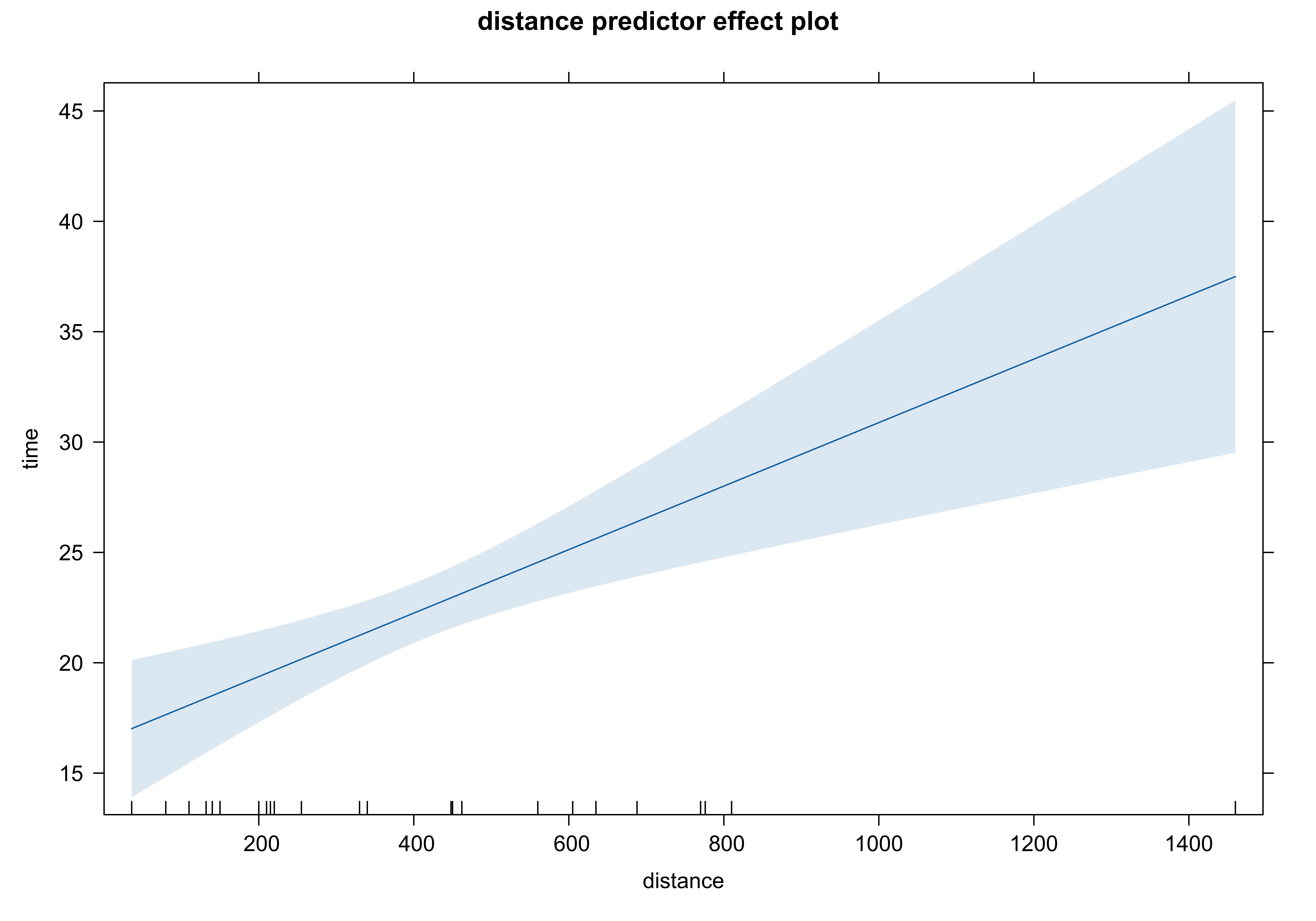
• Predictor effect plots look at 1 or 2D plots for each predictor.

• The predictor effect plot for \(x_1\):
  • fix the values of all other predictors ( \(x_2\) in the example)
  • substitute these fixed values into the fitted regression equation.
• Fix \(x_2\) at its average, \(\hat{y} = 2.34 + 1.62 ~x_1 + 0.014 (409.28)\)

• Same slope for any choice of fixed values of other predictors.

• The intercepts depend on the values of other predictors.

• A complete picture of the regression surface generated by the fitted model requires drawing a \(p\)-dimensional graph.

• Fix \(x_1\) at its average, \(\hat{y} = 2.34 + 1.62 (8.76) + 0.014 ~x_2\)

• The slope would be the same for any choice of fixed values of other predictors.

R Lab Predictor Effect Plots

library(effects)
plot(effects::predictorEffects(mod = delivery_lm))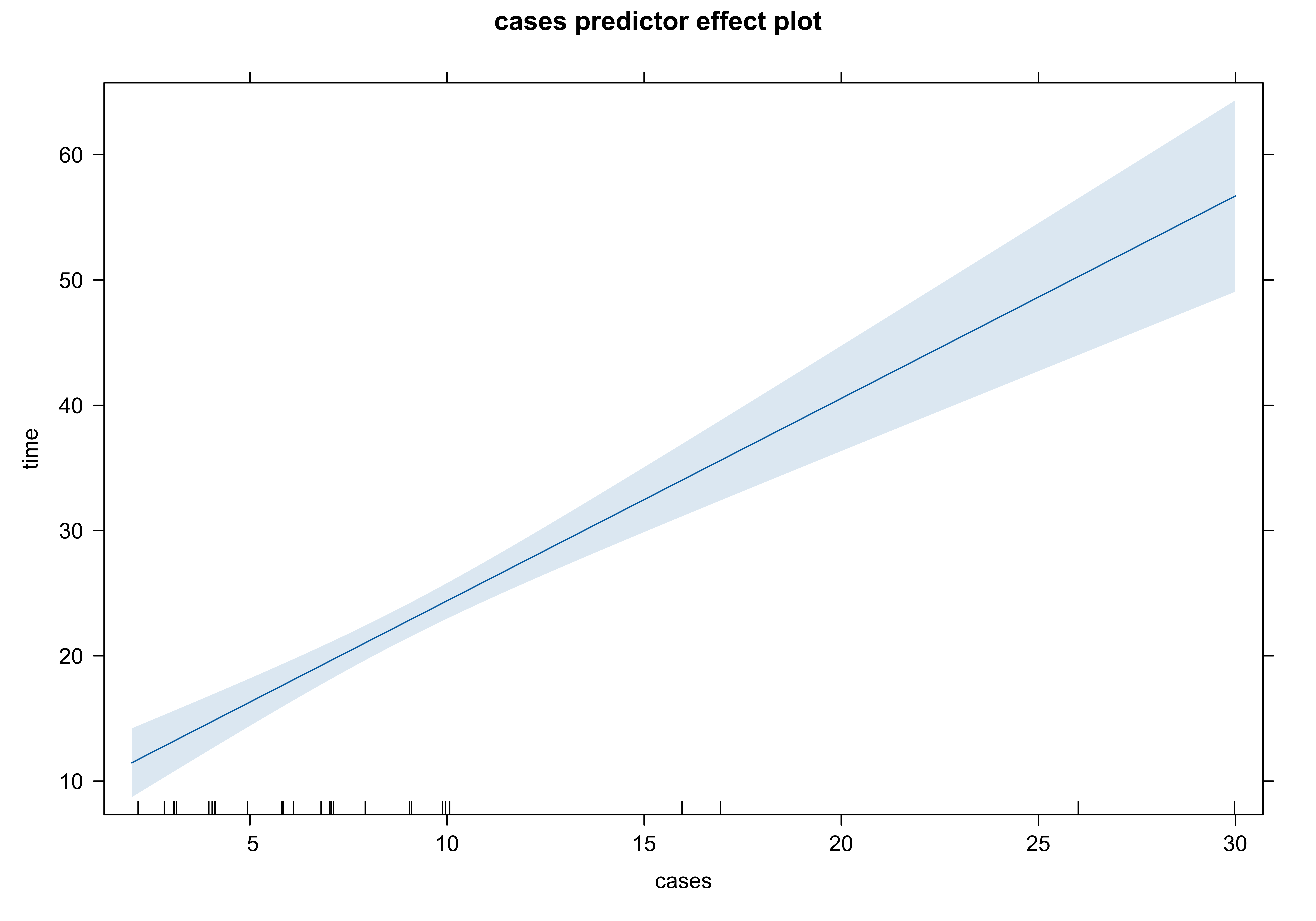

• rug plot
• the mean of time increases linearly as cases or distance increases.
• Given x2 variable in the model, what is the effect on x1 on the response.
• Without correction for simultaneous statistical inference
• plot(effects::predictorEffects(mod = delivery_lm, confint = list(type = “Scheffe”))) ‘arg’ should be one of “pointwise”, “Scheffe”, “scheffe”

Hypothesis Testing

Test for Significance of Regression

Tests on Individual Coefficients

Tests on Subsets of Coefficients (Later)

• Test for Significance: test if there is any regressor that has a significant effect on predicting \(Y\) or explaining the variation of \(Y\).
• In a Test for Significance, we are looking all the regressors.
• Tests on Individual Coefficients: we are only interested in single one predictor’s effect.
• But sometimes, we may be interested in a subset of Coefficients, not all, not single one, but two or three coefficients. And we’ll see how to do this kind of test later.
• Finally, we’ll learn the so-called General Linear Hypothesis that can perform a quite general test.
• The three tests above are in fact special case of the General Linear Hypothesis.

Test for Significance of Regression

• Test for significance: Determine if there is a linear relationship between the response and any of the regressor variables.
• \(H_0: \beta_1 = \beta_2 = \cdots = \beta_k = 0 \quad H_1: \beta_j \ne 0 \text{ for at least one } j\)

Source of Variation	SS	df	MS	F	\(p\)-value
Regression	\(SS_R\)	\(k\)	\(MS_R\)	\(\frac{MS_R}{MS_{res}} = F_{test}\)	\(P(F_{k, n-k-1} > F_{test})\)
Residual	\(SS_{res}\)	\(n-k-1\)	\(MS_{res}\)
Total	\(SS_{T}\)	\(n-1\)

• Reject \(H_0\) if \(F_{test} > F_{\alpha, k, n - k - 1}\).

• In SLR, test for significance is the same as testing individual coefficient \(\beta_1 = 0\).
• We may reject the null when the truth is all beta’s are nonzero, or only one single beta is nonzero.
• If there is only one nonzero beta, and we reject the null, basically, the nearly all the variation of Y is explained by the corresponding predictor that has the nonzero beta.
• We can still say the model is significant because that particular predictor has a significant effect on explaining y.
• Another way to represent SS_T

R Lab Test for Significance

\(H_0: \beta_{1} = \beta_{2} = 0 \quad H_1: \beta_j \ne 0 \text{ for at least one } j\)

summ_delivery

...
Coefficients:
            Estimate Std. Error t value Pr(>|t|)    
(Intercept)  2.34123    1.09673    2.13  0.04417 *  
cases        1.61591    0.17073    9.46  3.3e-09 ***
distance     0.01438    0.00361    3.98  0.00063 ***
---
Signif. codes:  0 '***' 0.001 '**' 0.01 '*' 0.05 '.' 0.1 ' ' 1

Residual standard error: 3.3 on 22 degrees of freedom
Multiple R-squared:  0.96,  Adjusted R-squared:  0.956 
F-statistic:  261 on 2 and 22 DF,  p-value: 4.69e-16
...

• How do we obtain the ANOVA Table?

R Lab Wrong ANOVA Table

Source of Variation	SS	df	MS	F	\(p\)-value
Regression	\(SS_R\)	\(k\)	\(MS_R\)	\(\frac{MS_R}{MS_{res}} = F_{test}\)	\(P(F_{k, n-k-1} > F_{test})\)
Residual	\(SS_{res}\)	\(n-k-1\)	\(MS_{res}\)
Total	\(SS_{T}\)	\(n-1\)

anova(delivery_lm) ## This is for sequential F-test

Analysis of Variance Table

Response: time
          Df Sum Sq Mean Sq F value  Pr(>F)    
cases      1   5382    5382   506.6 < 2e-16 ***
distance   1    168     168    15.8 0.00063 ***
Residuals 22    234      11                    
---
Signif. codes:  0 '***' 0.001 '**' 0.01 '*' 0.05 '.' 0.1 ' ' 1

• This is so called Type-I ANOVA table for a sequential F-test, which is NOT what we want.

R Lab ANOVA Table: Null vs. Full

Testing coefficients is like model comparison: Compare the full model with the model under \(H_0\)!

• Full model: including both cases and distance predictors
• Null model: no predictors \((\beta_1 = \beta_2 = 0)\)

## regression with intercept only
null_model <- lm(time ~ 1,
                 data = delivery_data)
anova(null_model, delivery_lm)

...
Analysis of Variance Table

Model 1: time ~ 1
Model 2: time ~ cases + distance
  Res.Df  RSS Df Sum of Sq   F  Pr(>F)    
1     24 5785                             
2     22  234  2      5551 261 4.7e-16 ***
...

• first row: info of SS_T
• second row: info of SS_R and SS_res
• does not show MS

\(R^2\) and Adjusted \(R^2\)

• \(R^2 = \frac{SS_R}{SS_T} = 1 - \frac{SS_{res}}{SS_T}\)
  • calculated as in SLR.
  • accesses how well the regression model fits the data.
  • measures the proportion of variability in \(Y\) that is explained by the regression or the \(k\) predictors.
  • The model with one additional predictor always gets a higher \(R^2\).

• There are other criterion or metrics for accessing model adequacy or model fit that may be better than R^2
• The model with one additional predictor always gets a higher \(R^2\) even the new predictor has no explanatory power or useless in predicting y. Because the predictor may capture the random noise variation, leading to decrease in \(SS_{res}\).
• If we use R^2 as the measure of model fit, then we will tend to include lots of regressors in the model, and we will always choose the model that has the most predictors, even though lots of predictors have no or little contribution to the fitting or prediction.
• The idea is a little bit like overfitting in machine learning.
• A complex or a larger model has several disadvantages.
  • First, it’s more difficult to interpret your model and results. It reduces the interpretability.
  • Second, the computing or running time is usually longer, and sometimes much longer depending on the order of complexity.
  • Also, the data or the model itself may consume lots of memory spaces.

Occam’s Razor: Don’t use a complex model if a simpler model can perform equally well!

• Adjusted \(R^2\)
  • \(R^2_{adj} = 1 - \frac{SS_{res}/(n-p)}{SS_T/(n-1)}\)
  • applies a penalty (through \(p\)) for number of variables included in the model.

• Not the more the better anymore
• Adjusted R2 doesn’t increase if the new variable does not provide very little information for prediction
• Adjusted R2 will only increase on adding a variable to the model if the addition of the regressor reduces \(MS_{res}\)
• This makes adjusted R2 a preferable metric for model selection in multiple regression models.

Adjusted \(R^2\) Example

• For a model with 3 predictors, \(SS_{res} = 90\), \(SS_T = 245\), and \(n = 15\). \[R^2_{adj} = 1 - \frac{90/(15-4)}{245/(15-1)} = 0.53\]
• The 4-th regressor is added into the model, and \(SS_{res} = 88\) (always decreases). Then \[R^2_{adj} = 1 - \frac{88/(15-5)}{245/(15-1)} = 0.49\]

Intuition: The new added regressor should have explanatory power for \(y\) large enough, so that \(MS_{res}\) is decreased.

R Lab \(R^2\) and Adjusted \(R^2\)

summ_delivery

...

Residual standard error: 3.3 on 22 degrees of freedom
Multiple R-squared:  0.96,  Adjusted R-squared:  0.956 
...

summ_delivery$r.squared

[1] 0.96

summ_delivery$adj.r.squared

[1] 0.96

Tests on Individual Regression Coefficients

• Hypothesis test on any single regression coefficient.
• \(H_0: \beta_{j} = 0 \quad H_1: \beta_j \ne 0\)
• \(t_{test} = \frac{b_j}{se(b_j)}\)
• Reject \(H_0\) if \(|t_{test}| > t_{\alpha/2, n-k-1}\)
• This is a partial or marginal test: a test of the contribution of \(X_j\) given ALL other regressors in the model.

• We can also do a one-side test for sure. But I am not sure if there is a R function to do a one-sided test.
• But we can always compute the test statistic or the p-value ourselves.
• Hypothesis test on any single regression coefficient.
• \(H_0: \beta_{j} = 0 \quad H_1: \beta_j \ne 0\)
• \(t_{test} = \frac{b_j}{\sqrt{\hat{\sigma}^2C_{jj}}}\), where \(C_{jj}\) is the \(j\)-th diagonal element of \(({\bf X'X})^{-1}\).
• Reject \(H_0\) if \(|t_{test}| > t_{\alpha/2, n-k-1}\)
• This is a partial or marginal test: a test of the contribution of \(X_j\) given ALL other regressors in the model.

R Lab Tests on Individual Coefficients

• Assess the value of \(x_2\) (distance) given that \(x_1\) (cases) is in the model.
• \(H_0: \beta_{2} = 0 \quad H_1: \beta_2 \ne 0\)

summ_delivery$coefficients

            Estimate Std. Error t value Pr(>|t|)
(Intercept)    2.341     1.0967     2.1  4.4e-02
cases          1.616     0.1707     9.5  3.3e-09
distance       0.014     0.0036     4.0  6.3e-04

qt(0.05/2, df = delivery_lm$df.residual, lower.tail = FALSE) ## t critical value df = n - 3 = 22

distance 
       4 

distance 
 0.00063 

Inference Pitfalls

• The test \(H_0:\beta_j = 0\) will always be rejected as long as the sample size is large enough, even \(x_j\) has a very small effect on \(y\).
  • Consider the practical significance of the result, not just the statistical significance.
  • Use the confidence interval to draw conclusions instead of relying only p-values.

• If the sample size is small, there may not be enough evidence to reject \(H_0:\beta_j = 0\).
  • DON’T immediately conclude that the variable has no association with the response.
  • There may be a linear association that is just not strong enough to detect given your data, or there may be a non-linear association.