Probability and Statistics 🎲

MATH 4780 / MSSC 5780 Regression Analysis

Dr. Cheng-Han Yu
Department of Mathematical and Statistical Sciences
Marquette University

Random Variables

Discrete Random Variables

• A discrete variable \(Y\) has countable possible values, e.g. \(\mathcal{Y} = \{0, 1, 2\}\)

• Probability (mass) function (pf or pmf) \[P(Y = y) = p(y), \,\, y \in \mathcal{Y}\]

  • \(0 \le p(y) \le 1\) for all \(y \in \mathcal{Y}\)

  • \(\sum_{y \in \mathcal{Y}}p(y) = 1\)

  • \(P(a < Y < b) = \sum_{y: a<y<b}p(y)\)

give an example.

Give me an example of a discrete variable/distribution!

Binomial Probability Function

\(P(Y = y; m, \pi) = \frac{m!}{y!(m-y)!}\pi^y(1-\pi)^{m-y}, \quad y = 0, 1, 2, \dots, m\)

Continuous Random Variables

• A continuous variable \(Y\) has infinite possible values, e.g. \(\mathcal{Y} = [0, \infty)\)

• Probability density function (pdf) \[f(y), \,\, y \in \mathcal{Y}\]

  • \(f(y) \ge 0\) for all \(y \in \mathcal{Y}\)

  • \(\int_{\mathcal{Y}}f(y) \, dy= 1\)

  • \(P(a < Y < b) = \int_{a}^bf(y)\,dy\)

Give me an example of continuous variable/distribution!

Normal (Gaussian) Density Curve

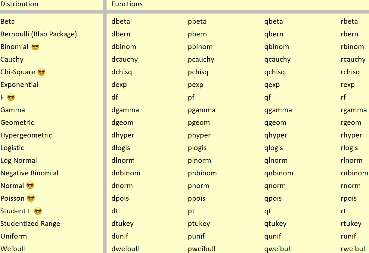
For continuous variables, \(P(a < Y < b)\) is the area under the density curve between \(a\) and \(b\).

Expected Value and Variance

For a random variable \(Y\),

• The expected value or mean: \(E(Y)\) or \(\mu\).

• The variance: \(\mathrm{Var}(Y)\) or \(\sigma^2\).

• The mean measures the center of the distribution, or the balancing point of a seesaw.

• The variance measures the mean squared distance from the mean, or dispersion of a distribution.

Discrete \(Y\):

\[E(Y) := \sum_{y \in \mathcal{Y}}yP(Y = y)\] \[\begin{align} \mathrm{Var}(Y) &:= E\left[(Y - E(Y))^2 \right] \\&= \sum_{y \in \mathcal{Y}}(y - \mu)^2P(Y = y)\end{align}\]

Continuous \(Y\):

\[E(Y) := \int_{-\infty}^{\infty}yf(y)\, dy\] \[\begin{align} \mathrm{Var}(Y) &:= E\left[(Y - E(Y))^2 \right] \\&= \int_{-\infty}^{\infty}(y - \mu)^2f(y)\, dy \end{align}\]

• The mean of a discrete random variable is the weighted average of possible values weighted by their corresponding probability.

• The variance of a discrete random variable is the weighted sum of squared deviation from the mean weighted by probability values.

• give an normal example

This is NOT the sample mean \(\overline{y}\) or sample variance \(s^2\).

If \(Y \sim binomial(n, \pi)\), what are the mean and variance?

R Lab dpqr Functions

For some distribution (dist),

• ddist(x, ...): density value \(f(x)\) or probability value \(P(X = x)\).
• pdist(q, ...): cdf \(F(q) = P(X \le q)\).
• qdist(p, ...): quantile of probability \(p\).
• rdist(n, ...): generate \(n\) random numbers.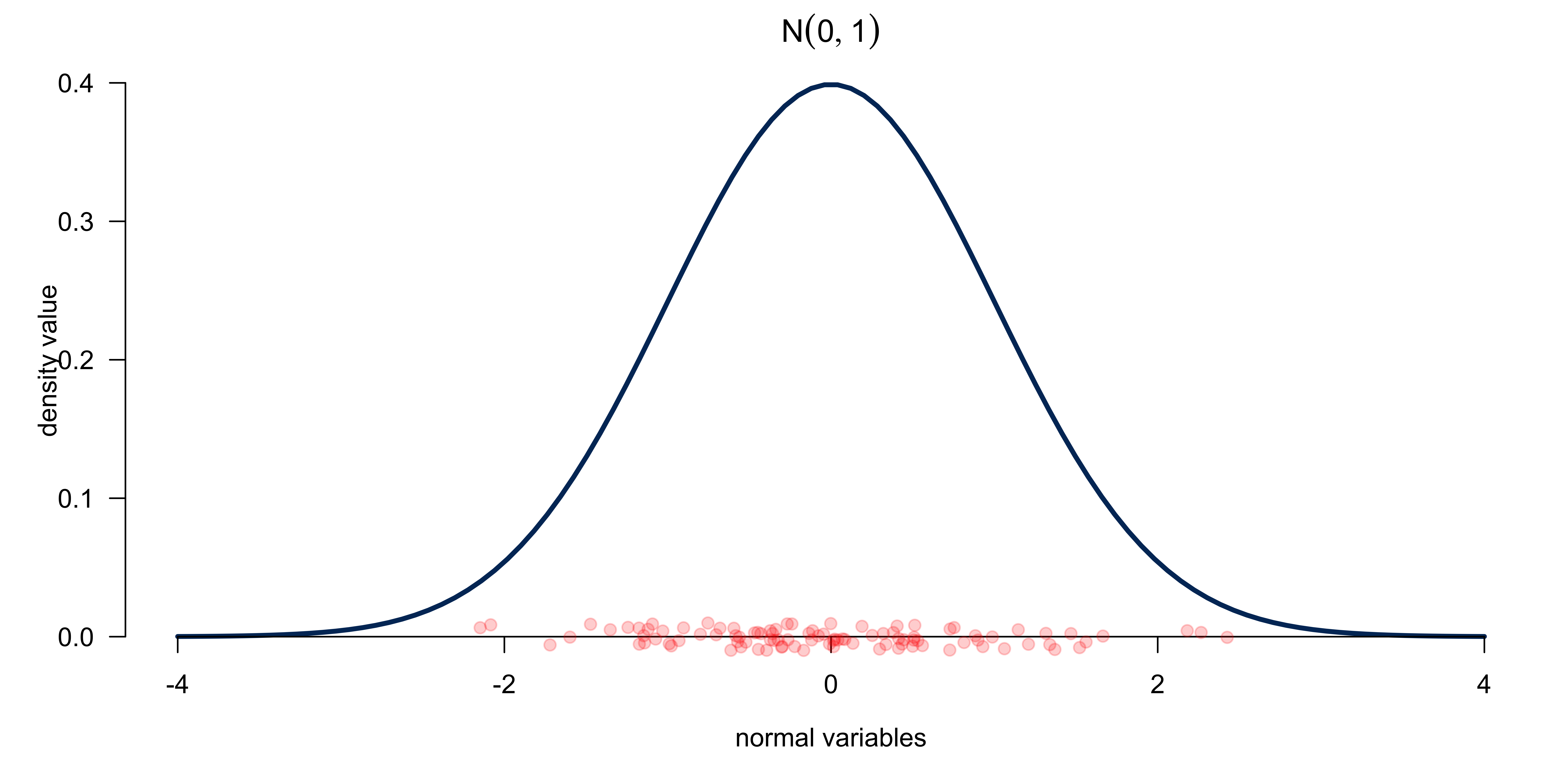

• In practice, we are not gonna calculate those properties by hand. Instead, we use computing software.
• In R we can use dpqr Functions to calculate probabilities or generate values from some distribution. Let’s see how.

## 10 binomial variable values with m = 5
rbinom(n = 10, size = 5, prob = 0.4)

 [1] 2 2 2 2 2 2 0 1 3 3

## P(X = 3) of binom(5, 0.4)
dbinom(x = 3, size = 5, prob = 0.4)

[1] 0.23

## P(X <= 2) of binom(5, 0.4)
pbinom(q = 2, size = 5, prob = 0.4)

[1] 0.683

R Lab dpqr Functions

## the default mean = 0 and sd = 1 (standard normal)
rnorm(5)

[1] -0.151  0.259 -0.649  0.846 -0.660

• \(100\) random draws from \(N(0, 1)\)

R Lab dpqr Functions

# P(0.5 < Z < 1) where Z ~ N(0, 1)
pnorm(1) - pnorm(0.5)

[1] 0.15

R Lab dpqr Functions

m <- 5
p <- 0.4
## mean
(mu <- sum(0:5 * dbinom(0:5, size = m, prob = p)))

[1] 2

m * p

[1] 2

## var
sum((0:5 - mu) ^ 2 * dbinom(0:5, size = m, prob = p))

[1] 1.2

m * p * (1 - p)

[1] 1.2

https://statisticsglobe.com/probability-distributions-in-r

Distributions

Some of Normals is Normal

• If \(Y \sim N(\mu, \sigma^2)\), \(Z = \frac{Y - \mu}{\sigma} \sim N(0, 1)\).

• If \(X \sim N(\mu_X, \sigma_X^2)\) and \(Y \sim N(\mu_Y, \sigma_Y^2)\) and \(X\) and \(Y\) are independent. Then for \(a, b \in \mathbf{R}\), \[aX + bY \sim N\left(a\mu_X+b\mu_Y, \color{red}{a^2} \color{black} \sigma_X^2 + \color{red}{b^2} \color{black} \sigma_Y^2\right)\]

What is the distribution of \(a_1Y_1 + a_2Y_2 + \cdots + a_nY_n\) if \(Y_i \sim N(\mu_i, \sigma^2_i)\) and \(Y_i\)s are independent?

• If \(Z \sim N(0, 1)\), then \[Z^2 \sim \chi^2_1\]

• If \(Z_i \stackrel{iid}{\sim} N(0, 1), i = 1, 2, \dots, k\), then \[\sum_{i=1}^k Z_i^2 \sim \chi^2_k\]

• \(iid\) means * independent identically distributed*.

• Let \(Y_i \stackrel{indep}{\sim} N(\mu_i, \sigma_i^2), i = 1, 2, \dots, n\). Then the random variable \(U = \sum_{i=1}^n a_iY_i\) has the distribution

Statistics Comes In

Suppose each data point \(Y_i\) of the sample \((Y_1, Y_2, \dots, Y_n)\) is a random variable from the same population whose distribution is \(N(\mu, \sigma^2)\), and \(Y_i\)s are independent each other: \[Y_i \stackrel{iid}{\sim} N(\mu, \sigma^2), \quad i = 1, 2, \dots, n\]

Statistics Comes In: Sampling Distribution

If \(Y_i \stackrel{iid}{\sim} N(\mu, \sigma^2), \quad i = 1, 2, \dots, n\),

• \(\overline{Y} \sim N\left(\mu,\frac{\sigma^2}{n} \right)\)

• \(Z = \frac{\overline{Y} - \mu}{\sigma/\sqrt{n}} \sim N(0, 1)\)

• Let the sample variance of \(Y\) be \(S^2 = \frac{\sum_{i=1}^n(Y_i - \overline{Y})^2}{n-1}\).

• \(\frac{\overline{Y} - \mu}{S/\sqrt{n}} \sim t_{n-1}\)

• Inference: \(\mu\) and \(\sigma^2\) are unknown, and \(\overline{y}\) and \(s^2\) are point estimates for \(\mu\) and \(\sigma^2\), respectively.

Why Use Normal? Central Limit Theorem (CLT)

• \(X_1, X_2, \dots, X_n\) are i.i.d. variables with mean \(\mu\) and variance \(\sigma^2 < \infty\).

• As \(n\) increases, the sampling distribution of \(\overline{X}_n = \frac{\sum_{i=1}^nX_i}{n}\) looks more and more like \(N(\mu, \frac{\sigma^2}{n})\), regardless of the distribution from which we are sampling \(X_i\)!

• Alright. We know why we want large sample. You will find that we use normal distribution quite often. It is not because it is called normal or more normal than other distributions. There is a reason why we use it.
• The reason is Central Limit Theorem.
• The CLT says that Suppose is \(\overline{X}_n\) is from a random sample of size \(n\) and from a population distribution having mean \(\mu\) and finite standard deviation \(\sigma\). As \(n\) increases, the sampling distribution of \(\overline{X}_n\) looks more and more like \(N(\mu, \sigma^2/n)\), regardless of the distribution from which we are sampling!
• Look at this figure. Your population distribution can be of any shape. As long as the distribution has mean and variance, its sampling distribution of sample mean will always look like a normal distribution as long as n is large.

Nature Methods 10, 809–810 (2013)

\((1-\alpha)100\%\) Confidence Interval for \(\mu\)

• \(T = \frac{\overline{Y} - \mu}{S/\sqrt{n}} \sim t_{n-1}\)

\[\small \begin{align} & \quad \quad P(-t_{\alpha/2, n-1} < T < t_{\alpha/2, n-1}) = 1 - \alpha \\ & \iff P(-t_{\alpha/2, n-1} < \frac{\overline{Y} - \mu}{S/\sqrt{n}} < t_{\alpha/2, n-1}) = 1 - \alpha \\ & \iff P(\mu-t_{\alpha/2, n-1}S/\sqrt{n} < \overline{Y} < \mu + t_{\alpha/2, n-1}S/\sqrt{n}) = 1 - \alpha \end{align}\]

\((1-\alpha)100\%\) Confidence Interval for \(\mu\): Probability

\[P\left(\mu-t_{\alpha/2, n-1}\frac{S}{\sqrt{n}} < \overline{Y} < \mu + t_{\alpha/2, n-1}\frac{S}{\sqrt{n}} \right) = 1-\alpha\]

Is the interval \(\left(\mu-t_{\alpha/2, n-1}\frac{S}{\sqrt{n}}, \mu + t_{\alpha/2, n-1}\frac{S}{\sqrt{n}} \right)\) our confidence interval?

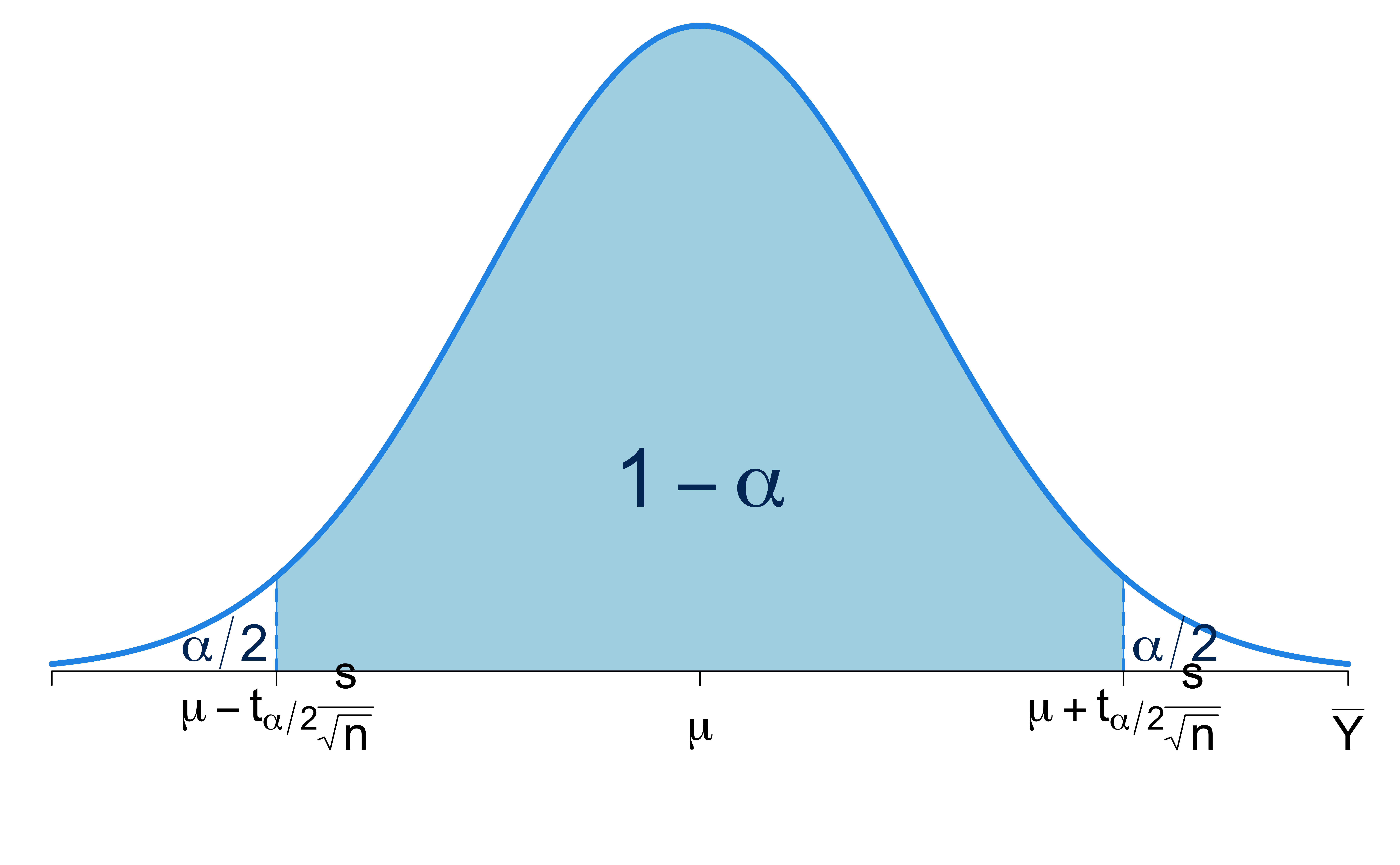
No! We don’t know \(\mu\), the quantity we’d like to estimate! But we almost there!

\((1-\alpha)100\%\) Confidence Interval for \(\mu\): Formula

\[\begin{align} &P\left(\mu-t_{\alpha/2, n-1}\frac{S}{\sqrt{n}} < \overline{Y} < \mu + t_{\alpha/2, n-1}\frac{S}{\sqrt{n}} \right) = 1-\alpha\\ &P\left( \boxed{\overline{Y}- t_{\alpha/2, n-1}\frac{S}{\sqrt{n}} < \mu < \overline{Y} + t_{\alpha/2, n-1}\frac{S}{\sqrt{n}}} \right) = 1-\alpha \end{align}\]

• With sample data of size \(n\), \(\left( \overline{y}- t_{\alpha/2, n-1}\frac{s}{\sqrt{n}}, \overline{y} + t_{\alpha/2, n-1}\frac{s}{\sqrt{n}} \right)\) is our \((1-\alpha)100\%\) CI for \(\mu\).

Hypothesis Testing

• \(H_0: \mu = \mu_0 \text{ vs. } H_1: \mu > \mu_0\), or \(\mu < \mu_0\), or \(\mu \ne \mu_0\)
• The significant level \(\alpha = P(\text{Reject } H_0 \mid H_0 \text{ is true}) = P(\text{Type I error})\)
• The test statistic is \(t_{test} = \frac{\overline{y} - \color{blue}{\mu_0}}{s/\sqrt{n}}\), a value from \(T \sim t_{n-1}\).
• When calculating a test statistic, we assume \(H_0\) is true.

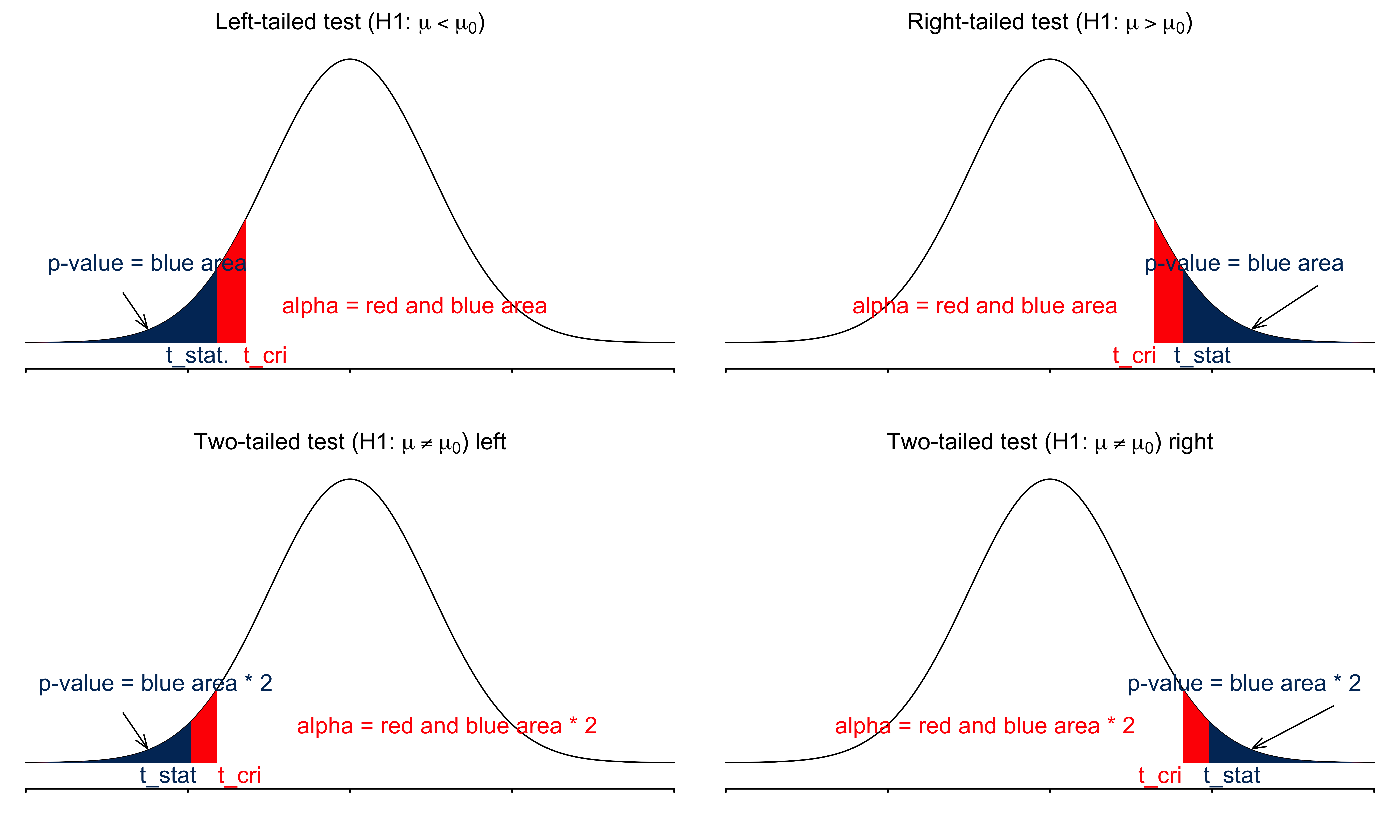
Reject \(H_0\) if

Method	Right-tailed \((H_1: \mu > \mu_0)\)	Left-tailed \((H_1: \mu < \mu_0)\)	Two-tailed \((H_1: \mu \ne \mu_0)\)
Critical value	\(t_{test} > t_{\alpha, n-1}\)	\(t_{test} < -t_{\alpha, n-1}\)	\(\mid t_{test}\mid \, > t_{\alpha/2, n-1}\)
\(p\)-value	\(\small P(T > t_{test} \mid H_0) < \alpha\)	\(\small P(T < t_{test} \mid H_0) < \alpha\)	\(\small 2P(T > \,\mid t_{test}\mid) \mid H_0) < \alpha\)

Both Methods Lead to the Same Conclusion