Exercise 2: Simple Linear Regression
Note
Simple Linear Regression
Basic Understanding
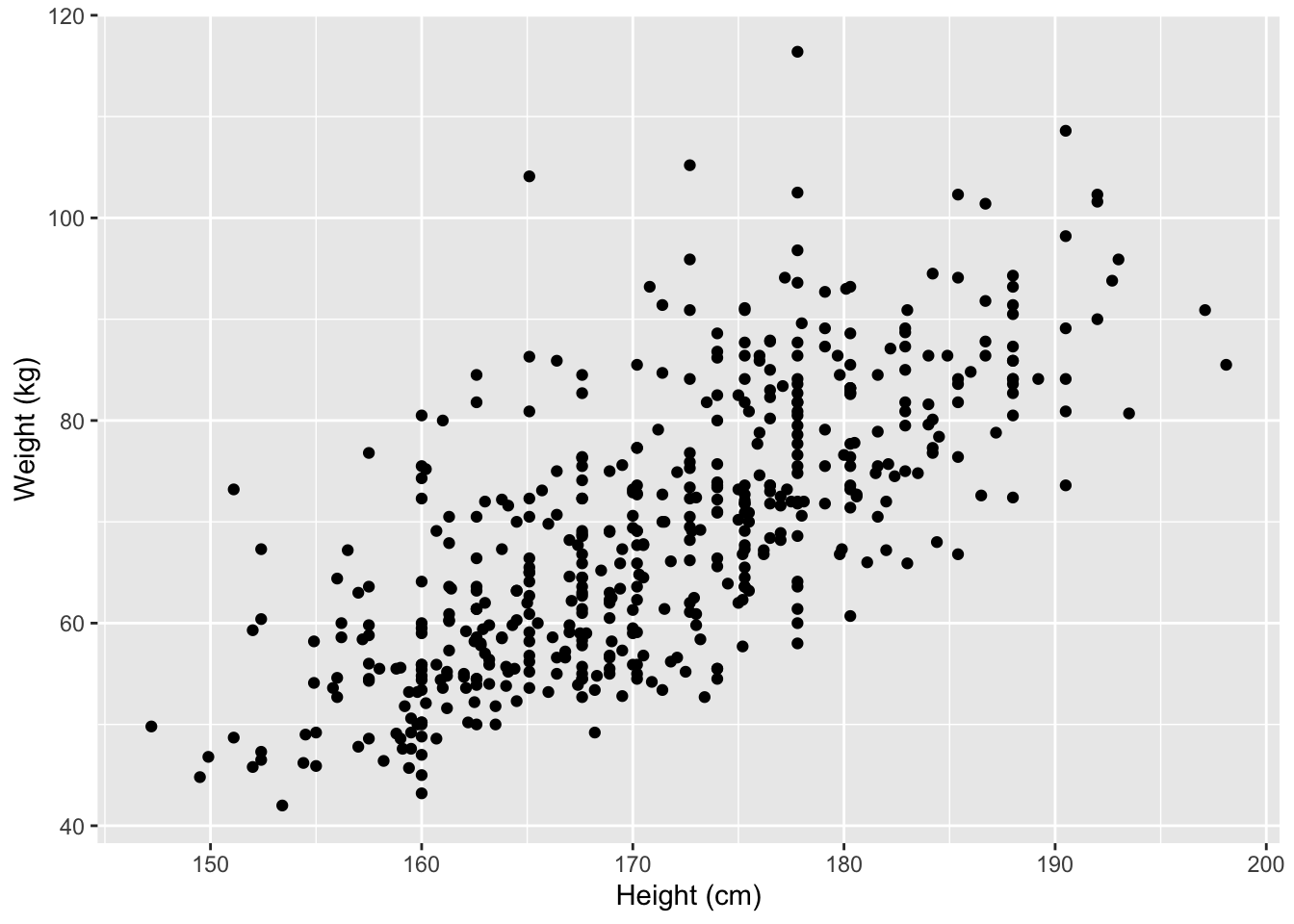
- The scatterplot and least squares summary below show the relationship between weight measured in kilograms and height measured in centimeters of 507 physically active individuals. (Heinz et al., 2003)

| term | estimate | std.error | statistic | p.value |
|---|---|---|---|---|
| (Intercept) | -105.01 | 7.54 | -13.93 | <0.0001 |
| hgt | 1.02 | 0.04 | 23.13 | <0.0001 |
Describe the relationship between height and weight.
Write the equation of the regression line. Interpret the slope and intercept in context.
Do the data provide convincing evidence that the true slope parameter is different than 0? State the null and alternative hypotheses, report the p-value, and state your conclusion.
The correlation coefficient for height and weight is 0.72. Calculate \(R^2\) and interpret it.
Simulation
- Generate a simulated data of size \(n = 100\) from the regression
\[y_i = 10 + 5x_i + \epsilon_i, ~~ \epsilon_i \stackrel{iid}{\sim} N(0, 2)\]
by completing the code
x <- runif(_____)
y <- ____ + ____ * ____ + r____(_____, sd = _____)
Fit a simple linear regression model to the data, then check whether the true slope is captured by the 90% confidence interval for the slope.